Hudson & Thames presents
LEARN MORE BY DOWNLOADING THE E-BOOK:
“THE DEFINITIVE GUIDE TO PAIRS TRADING”
INTRODUCTION
INTRODUCTION
Born at Morgan Stanley in the late 1980s, under the wing of Nunzio Tartaglia and his team, who later split up to start several of the world’s best hedge funds, namely PDT Partners and D.E. Shaw (which then lead to Two Sigma). Pairs trading has proven to be a popular and sophisticated trading strategy, often taught in advanced MSc Financial Engineering programs. A special mention to Gerry Bamberger who is the engineer that pioneered the technique and later left Morgan Stanley to join Ed Throp at Princeton Newport Partners.
With the rapid evolution of markets and advancement in technology, arbitrage opportunities have become scarcer and the margins – slimmer. To adapt to the market, the whole industry needed an upgrade! In the early 2000s, the once universally praised pairs trading strategy entered its “ice age” and after almost ten years, the resurgence of interest in the field brought numerous advanced approaches, and with that – the much-needed change.
The amount of advanced scientific research that has accumulated was exactly what was needed for the strategy to evolve and uncover its full potential as a truly universal and robust approach. The variety of methods range in complexity and choice of assets – this sets an entirely new stage for statistical arbitrage to shine in the current financial world.
From cointegration to copulas, this article gives you the ultimate guide on what pairs trading is today and why every market specialist has to pay attention to it.
WHAT IS PAIRS TRADING?
WHAT IS PAIRS TRADING?
First, we need to start with a definition of statistical arbitrage and pairs trading. Often people will use these two terms interchangeably, however, pairs trading is a subset of statistical arbitrage and so we can say that all pairs trading is statistical arbitrage but not all statistical arbitrage is pairs trading.
Statistical arbitrage is typically broken down into factor investing and the mean-reverting portfolios of pairs trading. We should add that in its simplest form pairs trading refers to trading only 2 assets but it can be extended to an n-dimensional mean reverting portfolio.
There is no single agreed-upon definition in the literature with each author bringing their own take, so we took it upon ourselves to formalize it as follows:
“Pairs trading is an approach that takes advantage of the mispricing between two (or more) co-moving assets, by taking a long position in one(many) and shorting the other(s), betting that the relationship will hold and that prices will converge back to an equilibrium level”
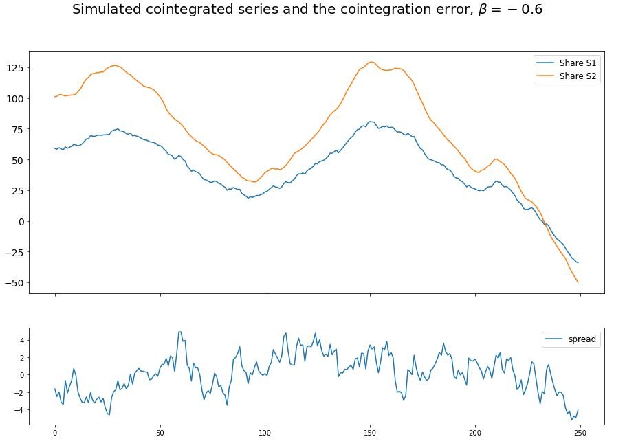
In the example below, we simulate a pair of co-moving assets using an implementation from ArbitrageLab. The first plot shows the co-moving assets whilst the bottom one illustrates how a mean-reverting spread is created by going long the first asset and short 60% in the second. It is this spread that can be traded without needing to make any forecasts about the future.
We will simulate the cointegrated pair and build a spread using the cointegration module from Arbitragelab.
The intuition behind pairs trading goes back to the fundamental principle of investing: “buy undervalued – and sell overvalued”. However, to determine if the asset is truly over or undervalued, we need to know the intrinsic value, which is at best an approximation and largely what value investing sets out to do.
Statistical arbitrage and pairs trading tries to solve this problem using price relativity. If two assets share the same characteristics and risk exposures, then we can assume that their behavior would be similar as well. This has the benefit of not having to estimate the intrinsic value of an asset but rather just if it is under or overvalued relative to a peer(s). We only have to focus on the relationship between the two, and if the spread happens to widen, it could be that one of the securities is overpriced, the other is underpriced, or the mispricing is a combination of both.
In this case, we are able to take advantage by selling the higher-priced security and buying the lower-priced one, expecting the mispricing to naturally correct itself in the future as prices converge to the equilibrium level.
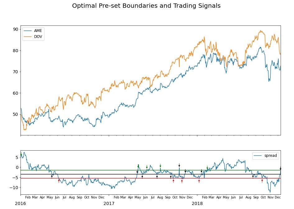
The example below shows the relationship between AME and DOV, notice how the spread is stationary enough for entry and exit positions to be taken and profits to be made.
An example of cointegration pairs trading strategy.
The mutual mispricing between the two assets is represented by the value of the spread. The greater the price difference from 0 and hence the spread, the greater the profit potential. One of the best qualities of pairs trading is market-neutrality, as by adjusting the hedge ratio of the spread it can be constructed to have a beta that is negligible, and therefore minimise the exposure to the market.
Pairs trading strategies usually vary in two ways: the way of detecting the “co-moving” pairs and the logic behind the trading rules. We dive into this topic in “A Taxonomy of Pairs Trading Strategies“.
THE HISTORY OF PAIRS TRADING
THE HISTORY OF PAIRS TRADING
It is hard to overestimate the influence that pairs trading has had on the industry. The initial members of the team consisted of mathematicians and physicists under Nunzio Tartaglia, who later branched off to establish such renowned independent practitioners as D.E. Shaw and PDT Partners, just to name a few. Many stories from the golden era of statistical arbitrage, about the business and its practitioners, have been mythologized by the industry.
For example how the SEC came to use algorithms from Morgan Stanley’s Black Box to detect atypical price patterns or the gradual embrace of the technique by the independent specialists and later the practice of “bandwagoning” of the weak stock accumulation by the “big house”.
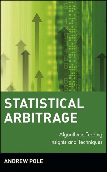
As the information spread to a broader audience and the power of low-cost personal computers started to rise rapidly, the number of pairs trading practitioners rose as well. After two decades of prosperity, the swift evolution of the market called for an upgrade in approaches. It caused a significant diminish in returns for pairs trading when compared to the early days. Managers were struggling to adapt the strategies to the new reality and as a result, gradually started to withdraw investments. In his book “Statistical Arbitrage: Algorithmic Trading Insights and Techniques”, Andrew Pole called this the “ice age” of statistical arbitrage. Similar to the actual “ice age”, it didn’t last forever.
“I considered titling the book, The Rise and Fall and Rise? of Statistical Arbitrage, reflecting the history and the possibilities now emerging.”
– Andrew Pole
Time was exactly what was needed for the ice to melt and give pairs trading its long-awaited new beginning. Ten years later the interest of the research community sparked yet again turning into the bright fire of technological advancement and continuous research in the field. As research in pairs trading continued to accumulate, it evolved into a truly versatile approach with a variety of frameworks with different complexity and empirical applications across various asset classes.
Numerous advances in techniques are continuously being added to our codebase as new research is released. This makes ArbitrageLab a perfect tool for investment managers who want to hit the ground running.
3 STEPS TO BUILD A PAIRS TRADING STRATEGY
3 STEPS TO BUILD A PAIRS TRADING STRATEGY
GETTING STARTED WITH THE BASICS
GETTING STARTED WITH THE BASICS
RECOMMENDED LITERATURE
RECOMMENDED LITERATURE
PAIRS TRADING LECTURES SERIES
PAIRS TRADING LECTURES SERIES
PAIRS TRADING IN VARIOUS MARKETS
PAIRS TRADING IN VARIOUS MARKETS
Previously we’ve discussed the “what’s” and “why’s” of pairs trading. Now it’s time to move on to the question of “where?”. Where do we apply pairs trading strategies? Building a strategy starts with pair selection, so our desire to choose the best market for it is only natural.
Since pairs trading bears its roots in equity markets, it usually serves as the first pick by most traders, this is largely due to the high number of possible combination pairs. However, asset classes such as commodities, forex, or even crypto have numerous supporting studies on the profitability of statistical arbitrage. Some have been around since 1990, as is the case for commodities futures; some are more recent, like crypto markets, however, they all support the universality of statistical arbitrage.
The requirement of “price co-movement” and “short-term price inefficiency” can be applied to every conceivable type of asset. Whether it’s ETFs or options, if the market exhibits the violation of the “Law of One Price”, statistical arbitrage will thrive.
With every market and every asset at our disposal, we need to be aware of the nuances that come with given asset types and how they influence our approach to strategy creation.
EQUITY & ETF
EQUITY & ETF
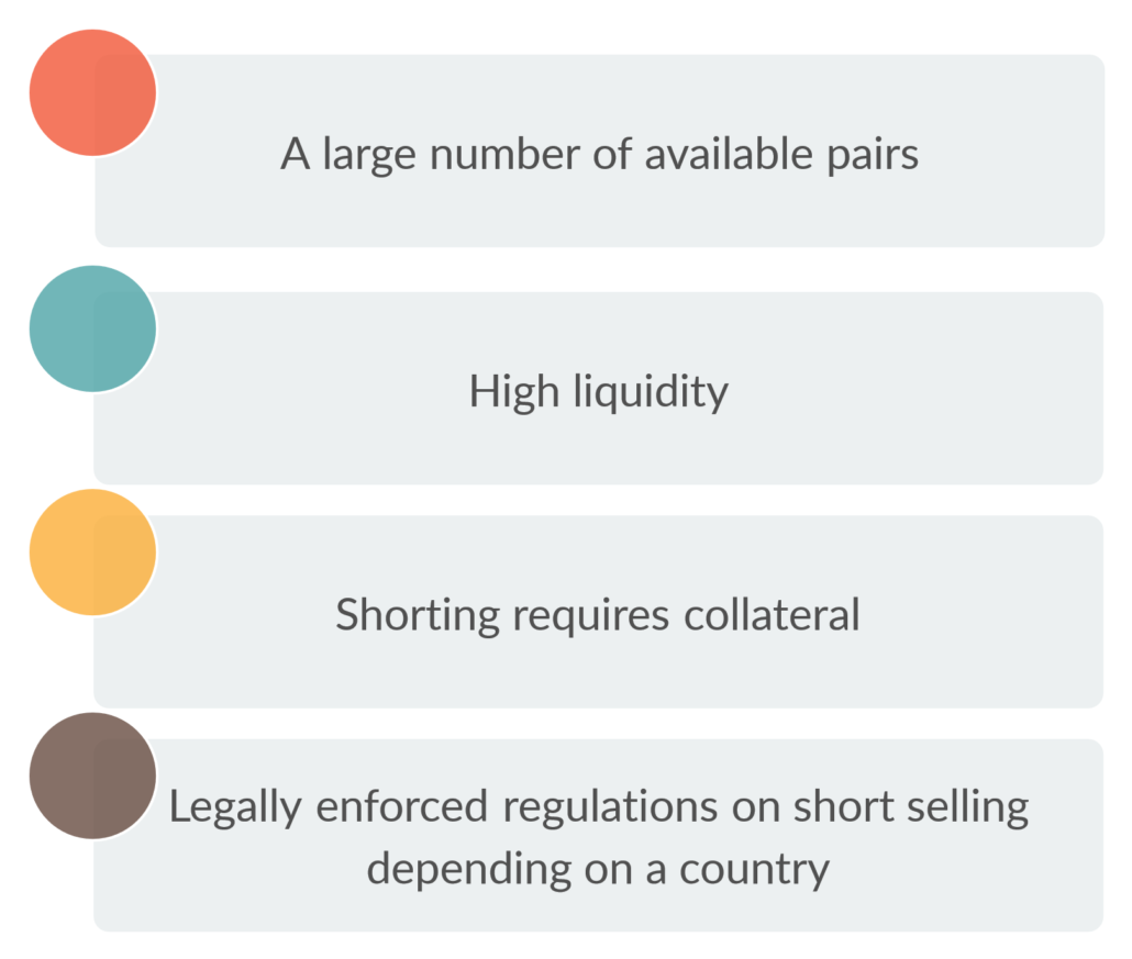
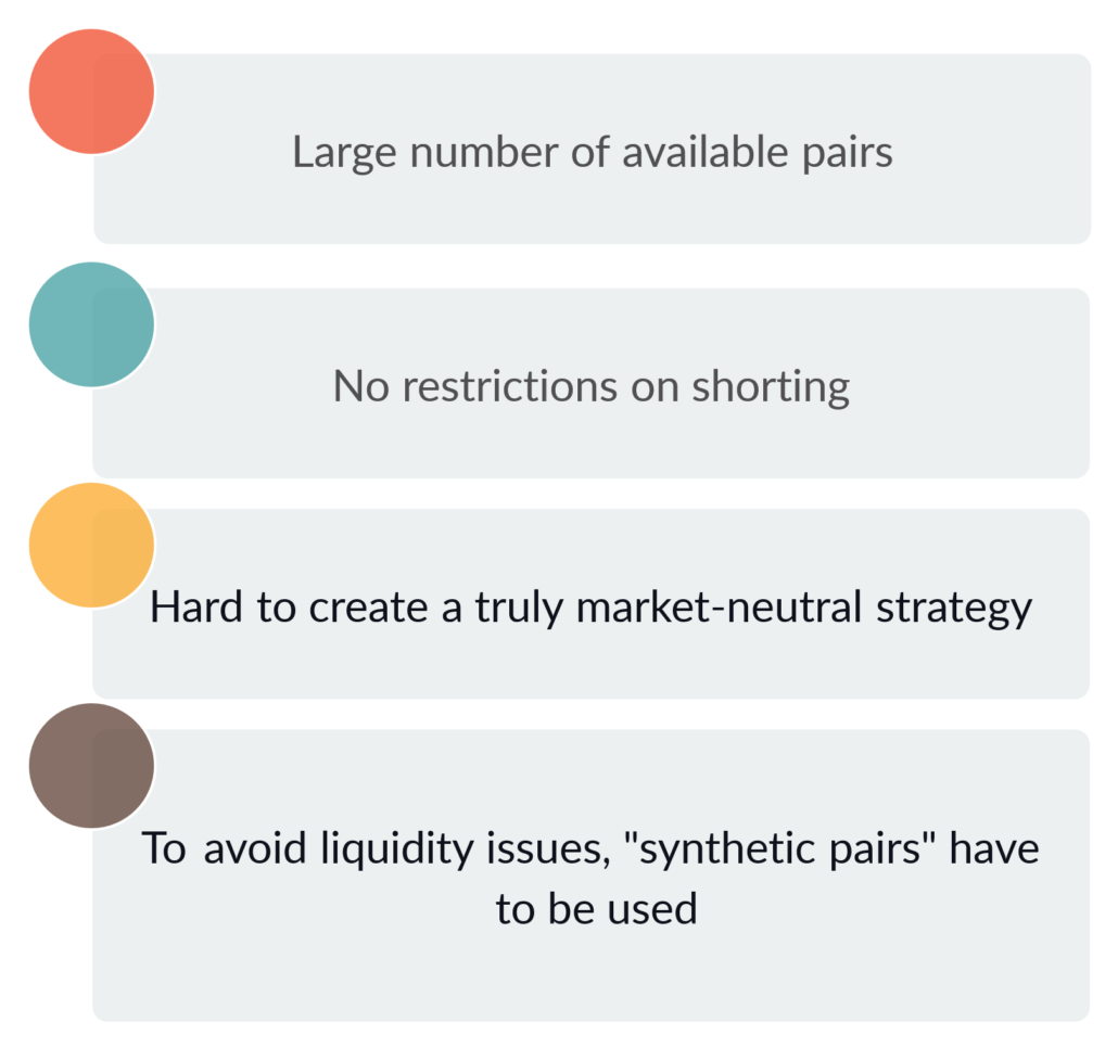
This is the first choice for most traders as it allows for the highest number of combination pairs. The study by Jacobs & Weber conducted on 34 international markets has empirically proven that pairs trading is the most profitable in emerging markets, either due to the higher inefficiencies, or markets with a large number of pairs. However, with the benefits of the stock and ETF markets come their limitations. Shorting is vital for statistical arbitrage strategies, so as the investor, we need to be aware of the market’s requirements to be able to perform them. Applying statistical arbitrage strategies to equity or ETFs, we need to take into account three main points. First – short selling these types of assets requires collateral. Second – the less popular the stock or the ETF, the harder it is to find a willing lender to make the short possible, and third – legal restrictions on shorting can exist in different countries. An example of the latter could be “The uptick rule.” previously used in the US stock market, or the short sale ban that existed in Chinese stock market.
FUTURES
FUTURES
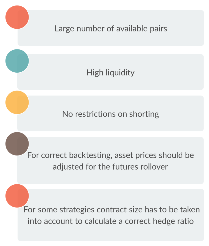
Futures, and commodities futures specifically, are also no stranger to pairs trading. The phenomenon of price co-movement for the raw commodities, essential for statistical arbitrage, was discovered by studies as far as three decades ago. The advantage of choosing futures also has to do with shorting, as no additional requirements have to be fulfilled to perform the short sell. The nuances lie in the technical details connected with strategy backtesting or spread creation. First and foremost, the backtesting data has to be adjusted for the futures roll to simulate the correct PnL path. However, to size positions and determine capital consumption, we have to use raw prices. For some pairs trading strategies, it is also important to account for contract size and implied volatility to determine the correct hedging ratio.
FOREX
FOREX
The forex market is not the most popular choice for statistical arbitrage, but still, a fair share of traders utilize pairs trading strategies using currency pairs. To create the desired spread, one would use a technique called “synthetic pairs”. The goal is to avoid a situation where directly trading the currency is impossible due to low liquidity, as provided by the broker. To do so, the institutional trader places two separate offsetting trades of target currencies with one highly trading currency(usually USD) acting as the intermediary(example: AUD/USD and USD/CAD). Another advantage of the forex market is the fact that shorting is as easy as selling the corresponding currency pair.
CRYPTO
CRYPTO
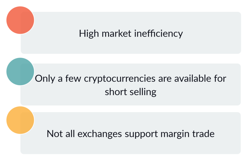
Despite being the youngest and having less research than previously mentioned assets, the cryptocurrency market is very attractive for statistical arbitrage, from a theoretical standpoint. Al-Yahyaee et al. found that Bitcoin’s inefficiency is higher than stocks or forex markets, indicating that trading might have an even greater potential to be profitable here than elsewhere. However, the main limitation for crypto traders today is that only a few of the top traded coins are available for short-selling, and not all exchanges provide you with the option to do so. Additionally, transaction costs from brokers in the form of commissions and spreads can be larger than in more established markets such as equities.
A TAXONOMY OF PAIRS TRADING STRATEGIES
A TAXONOMY OF PAIRS TRADING STRATEGIES
The pairs trading literature significantly grew its conceptual framework and empirical application base when the interest of the research community was sparked once again in the late 2010-s and continues to fuel the research till this day. As a large amount of literature on statistical arbitrage strategies accumulated – the necessity for classification arose.
Krauss(2015) recognizes 5 types of approaches:
- Distance approach
- Cointegration approach
- Time series approach
- Stochastic control
- Other: consisting of PCA, copula, and Machine Learning approaches.
Let’s take a deeper look into the taxonomy of pairs trading strategies.
DISTANCE APPROACH
DISTANCE APPROACH
Popularized by Gatev in 2006, this approach holds the position of the most cited pairs trading strategy. The simplicity and transparency of this method make it the first choice when it comes to large empirical research.
Main idea:
During the pair selection process, various distance metrics like pearson’s correlation, distance correlation, angular distance, and so on, are leveraged to identify the co-moving securities. In the trading period, simple nonparametric threshold rules are used to trigger the trading signals.
COINTEGRATION APPROACH
COINTEGRATION APPROACH
Another extremely popular approach outlined by Vidyamurthy 2004, is the cointegration approach. Pairs selected in this method possess econometrically more reliable equilibrium relationships.
Main idea:
The pairs selection process is conducted by applying a cointegration tests to identify co-moving assets. Trading signals are generated by using simple rules, mostly generated by (Gatev et al 2006) threshold rules.
TIME SERIES APPROACH
TIME SERIES APPROACH
To improve the trading rules of a given strategy, we turn to time series modeling of a mean-reverting process, other than cointegration.
Main idea:
During the pairs selection step our goal is to create a truly mean-reverting portfolio/spread. The mean-reverting process of choice is fitted to the spread, in order to determine the optimal rules for the trading strategy. One of the most popular mean-reverting processes used in the literature is the Ornstein-Uhlenbeck process.
STOCHASTIC CONTROL APPROACH
STOCHASTIC CONTROL APPROACH
By using stochastic processes we can determine the optimal trading rules for a given mean-reverting strategy, without the need to forecast how the spread will move in the next period or needing a formation period.
Main idea:
This is an advanced pairs trading strategy that relies on using stochastic processes to generate the optimal trading rules and policies for mean reverting portfolios.
OTHER APPROACHES
OTHER APPROACHES
Although grouped as “other”, the approaches contained in this bucket are one of the most advanced in the field, we will look at them one by one and expand on their differences.
COPULA
The Copula approach allows you to study the deeper relationship between the different legs of the trade and enables you to analyze the dependency structure from multiple random variables. This novel approach also allows you to work with multiple assets rather than only working with a single pair (2 assets). The trading rules selection process usually relies on the concept of conditional probability. The data fitting process for copulas is usually divided into two parts: translating marginal data into quantiles and fitting a copula with the following quantiles.
PCA
The approach proposed by Avellaneda and Lee (2010) uses PCA to create a seemingly mean-reverted spread which in turn is modeled by an OU-process. The trading rules are generated similarly to the time series approach, and the main focus is on the type of principal component analysis method utilized – asymptotic, regular, or a multivariate cointegration model. This model, at the time of writing, is considered by many to be the cutting edge of mean reversion trading.
MACHINE LEARNING
The machine learning approach is characterized by utilizing the techniques used in different approaches in combination with machine learning algorithms and applying them to strategy creation process.
Whilst forecasting time series is a hard problem, and non-linear models show a lot of promise, we instead choose to focus on machine learning for pairs selection. The book “A Machine Learning based Pairs Trading Investment Strategy” by Sarmento and Horta provides a sophisticated and well thought out process to determine high-quality pairs. You can read all about it here: Employing Machine Learning for Pairs Selection.
BACKTESTING THE STRATEGY
BACKTESTING THE STRATEGY
“Backtesting is not a research tool. Feature importance is.“
– Marcos Lopez De Prado
In his book Advances in Financial Machine Learning, Prof. Marcos Lopez de Prado defines the process of backtesting as a “Historical simulation of how a strategy would have performed should it have been run over a past period of time”. It means that backtesting doesn’t provide us with the tools to deduce a precise cause-effect relationship akin to what feature engineering does. We can’t guarantee that the Sharpe ratio achieved can be replicated if we travel back in time.
3 KEY BACKTESTING METHODS
3 KEY BACKTESTING METHODS
The Walk-Forward Method
The walk-forward method is the most commonly used method in the industry. In this approach, the testing moves forward in time with the goal of preventing leakage from look-ahead information and can simply be thought of as a historical simulation / historical backtesting. This method assesses the performance of an investment algorithm under the assumption that history repeats itself exactly. However, it doesn’t account for the randomness of the data-generating process. It only accounts for a single historical path.
The Resampling Method
The resampling method addresses the weakness of the walk-forward technique, by introducing the assumption that future paths can be simulated by resampling of past observations. The resampling methods can vary from deterministic (jackknife, cross-validation) to random (subsampling, bootstrap). The ability to produce different paths in return allows us to do things like bootstrapping the Sharpe ratio distribution, which was impossible with a single path simulation. In addition, it is more difficult to overfit a resampling backtest than the walk-forward one. And yet there is still a possibility that resampling from a finite historical sample may not be representative of the future.
The Monte-Carlo Method
This approach improves on what the previous two were lacking – a deeper understanding of the data generation process. It assesses the algorithm’s performance under the assumption that future paths can be simulated via Monte Carlo and relies on knowledge derived from the statistical analysis of the observations or theory (market microstructure, institutional processes, economic links, etc.). An example from Lopes de Prado: ”For instance, economic theory may suggest that two variables are cointegrated, and empirical studies may indicate the range of values that characterize the cointegration vector. Accordingly, researchers can simulate millions of years of data, where the cointegration vector takes many different values within the estimated range.This is a much richer analysis than merely resampling observations from a finite (and likely unrepresentative) set of observations (see Advances in Financial Machine Learning, chapter 13)”
NUANCES OF BACKTESTING
NUANCES OF BACKTESTING
Backtesting is important for every strategy, however, it usually leads to overfitting and false investment discovery. The hope is that if done properly, it provides us with necessary insight to validate or discard the results of our research. Hence, it comes without saying that you have to be attentive to the nuances that come with the type of strategy you are using. Overlooking such details can render the whole procedure useless, even if all our assumptions are flawless and we account for every possible bias.
It is for this reason that the best researchers and practitioners advocate for the use of performance metrics not derived from a backtest. A good example of this is the ROC, and confusion matrices generated from classification models.
One particular problem that comes up when trying to backtest strategies that use futures contracts is adjusting for the roll and another is that the typical vectorized backtest methodology doesn’t work when backtesting a strategy that has multiple long and short positions, as it is in mean reverting portfolios (pairs trading). A good example of this is our informative article on The Correct Vectorized Backtest Methodology for Pairs Trading. In the article, we highlight common pitfalls and how to correctly generate an equity curve / PnL plot.
CONCLUSION
CONCLUSION
Pairs trading is a truly versatile class of trading strategies that harbours enormous potential. ArbitrageLab is a collection of the landmark and most cutting edge implementations all packaged into a python library, making it perfect for investors who want to hit the ground running. The Comprehensive Introduction to Pairs Trading was created to answer the questions arising whilst building these strategies.
Starting from the basics, we covered the history of pairs trading, potential benefits and nuances of different asset classes to trade, the taxonomy of a Pairs Trading Strategy, and finally notes on backtesting and a walk-forward backtesting framework to help you in your journey to construct the ultimate pairs trading strategy.
To dive into our latest research on constructing mean-reverting portfolios click here.
REFERENCES
- Al-Yahyaee, K.H., Mensi, W. & Yoon, S.-M., 2018. Efficiency, multifractality, and the long-memory property of the Bitcoin market: A comparative analysis with stock, currency, and gold markets. Finance Research Letters, 27, pp.228–234.
- Anon, 2015. Arbitrage and Pairs Trading. The Handbook of Pairs Trading, pp.89–95.
- Chan, E., 2013. Algorithmic Trading: Winning Strategies and Their Rationale, John Wiley & Sons.
- Ehrman, D.S., 2006. The handbook of pairs trading: strategies using equities, options, and futures, John Wiley & Sons.
- Elliott, R.J., *, J.V.D.H. & Malcolm, W.P., 2005. Pairs trading. Quantitative Finance, 5(3), pp.271–276.
- Endres, S. & Stübinger, J., 2019. Optimal trading strategies for Lévy-driven Ornstein–Uhlenbeck processes. Applied Economics, 51(29), pp.3153–3169.
- Fil, M. & Kristoufek, L., 2020. Pairs Trading in Cryptocurrency Markets. IEEE Access, 8, pp.172644–172651.
- Gatev, E., Goetzmann, W.N. & Rouwenhorst, K.G., 2006. Pairs Trading: Performance of a Relative-Value Arbitrage Rule. Review of Financial Studies, 19(3), pp.797–827.
- Hagen, J.V., 1989. Relative Commodity Prices and Cointegration. Journal of Business & Economic Statistics, 7(4), pp.497–503.
- Jacobs, H. & Weber, M., 2015. On the determinants of pairs trading profitability. Journal of Financial Markets, 23, pp.75–97.
- Krauss, C., 2016. Statistical Arbitrage Pairs Trading Strategies: Review And Outlook. Journal of Economic Surveys, 31(2), pp.513–545.
- Liew, R.Q. & Wu, Y., 2013. Pairs trading: A copula approach. Journal of Derivatives & Hedge Funds, 19(1), pp.12–30.
- Mavrakis, E. & Alexakis, C., 2018. Statistical Arbitrage Strategies under Different Market Conditions: The Case of the Greek Banking Sector. Journal of Emerging Market Finance, 17(2), pp.159–185.
- Pole, A., 2007. Statistical arbitrage: algorithmic trading insights and techniques, John Wiley & Sons.
- Prado, M.L.de, 2018. Advances in Financial Machine Learning, Wiley.
- Prado, M.L.D., 2019. Tactical Investment Algorithms. SSRN Electronic Journal.
- Ramos-Requena, J.P., Trinidad-Segovia, J.E. & Sánchez-Granero, M.Á., 2020. Some Notes on the Formation of a Pair in Pairs Trading. Mathematics, 8(3), p.348.
- Vidyamurthy, G., 2011. Pairs Trading: Quantitative Methods and Analysis, John Wiley & Sons, Inc.


