Model Interpretability: The Model Fingerprint Algorithm

By Oleksandr Proskurin

Model Fingerprint (Li, Y., Turkington, D. and Yazdani, A., 2020)

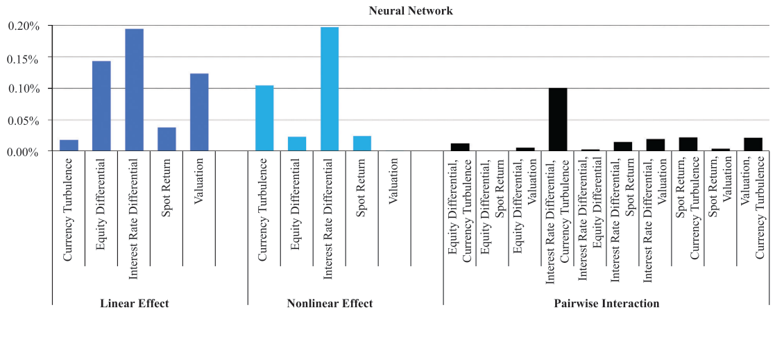
“The complexity of machine learning models presents a substantial barrier to their adoption for many investors. The algorithms that generate machine learning predictions are sometimes regarded as a black box and demand interpretation. Yimou Li, David Turkington, and Alireza Yazdani present a framework for demystifying the behaviour of machine learning models. They decompose model predictions into linear, nonlinear, and interaction components and study a model’s predictive efficacy using the same components. Together, this forms a fingerprint to summarize key characteristics, similarities, and differences among different models.” [2]

One of the key principles in financial machine learning is:

“Backtesting is not a research tool. Feature importance is.” (Dr. Marcos Lopez de Prado)

The research guided by feature importance helps us understand the effects detected by the model. This approach has several advantages:

The research team can improve the model by adding extra features which can describe patterns in the data. In this case, adding features is not a random generation of various technical and fundamental indicators, but rather a deliberate process of adding informative factors.
During drawdown periods, the research team would want to help explain why a model failed and some degree of interpretability. Is it due to abnormal transaction costs, a bug in the code, or is the market regime not suitable for this type of strategy? With a better understanding of which features add value, a better answer to drawdowns can be provided. In this way models are not as ‘black box’ as previously described.
Being able to interpret the results of a machine learning model leads to better communication between quantitative portfolio manager and investors. Clients feel much more comfortable when the research team can tell a story.

There are several algorithms used to generate feature importances for various types of models.

Mean Decrease Impurity (MDI). This score can be obtained from tree-based classifiers and corresponds to sklearn’s feature_importances attribute. MDI uses in-sample (IS) performance to estimate feature importance.
Mean Decrease Accuracy (MDA). This method can be applied to any classifier, not only tree-based. MDA uses out-of-sample (OOS) performance in order to estimate feature importance.
Single Feature Importance (SFI). MDA and MDI each suffer from substitution effects: if two features are highly correlated, one of them will be considered as important while the other one will be redundant. SFI is an OOS feature importance estimator which doesn’t suffer from substitution effect because it estimates each feature importance separately.

Recently, we found a great article in a Journal of Financial Data Science:Beyond the Black Box: An Intuitive Approach to Investment Prediction with Machine Learning. By Yimou Li, David Turkington and Alireza Yazdani. Which provides a technique for feature importance by breaking any model down to its linear, non-linear and pairwise interaction effects for each feature. In this way, each model has a type of “fingerprint”.

The Model Fingerprints Algorithm

Let’s discuss at a high level the idea of the Fingerprints algorithm. For each feature $X_i$ in a dataset we loop through possible feature values ${x_k}$ and generate an average model prediction whilst keeping the other features fixed. As a result, for each feature $k$ we have a set of x values and corresponding average prediction when feature values are fixed. This dependency is known as the partial dependence function $f_k(x)$

The partial dependence function provides an intuitive sense for the marginal impact of the variable of interest, which we may think of as a partial prediction. The partial dependence function will have small deviations if a given variable has little influence on the model’s predictions. Alternatively, if the variable is highly influential, we will observe large fluctuations in prediction based on changing the input values. [2]

Estimating linear/non-linear effect

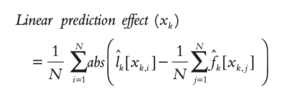
In order to estimate linear and non-linear effect, for each feature we first fit a regression line for the partial dependence function. The regression line for feature $k$ is denoted as $l_k[x_{k,j}]$ . The authors of the paper define the linear effect as the mean absolute deviations of the regression line predictions around their partial dependence function.

The non-linear effect is defined as the mean absolute deviation of the total marginal (single variable) effect around its corresponding linear effect. [2]

Estimating pairwise interaction effect

In order to estimate pairwise effect, we need to fix both feature values and generate partial dependence function value for a pair of feature values $x_i, x_j$ . Interaction effect is defined as demeaned joint partial prediction of the two variables minus the demeaned partial predictions of each variable independently.

Why The Model Fingerprints Algorithm ?

The Model Fingerprint gives us the information not only about feature importance, but also how feature values influence model predictions. Does volatility have a low linear effect, but a high non-linear impact? Can it explain poor algorithm performance during range periods? How informative is 50-day volatility in a pair with the RSI indicator? Maybe a volume change itself is not that informative however in pair with price change it has high interaction effect. The algorithm not only highlights important features but also explains the nature of feature importance. This information can be used to better enable research to create future research roadmaps, feature generation plans, risk-models, etc.

The Model Fingerprints algorithm was implemented in the latest mlfinlab release. In this post we would like to show how MDI, MDA, SFI feature importance and Model Fingerprints algorithms can give us an intuition about a Trend-Following machine learning model.

Trend-Following example

Import modules

import numpy as np
import pandas as pd
import timeit

from sklearn.ensemble import RandomForestClassifier, BaggingClassifier
from sklearn.metrics import roc_curve, accuracy_score, precision_score, recall_score, f1_score, log_loss
from sklearn.tree import DecisionTreeClassifier
import matplotlib.pyplot as plt

import mlfinlab as ml
from mlfinlab.feature_importance import (mean_decrease_impurity, mean_decrease_accuracy, single_feature_importance, plot_feature_importance)
from mlfinlab.feature_importance import ClassificationModelFingerprint

Read the data, generate SMA crossover trend predictions

# Compute moving averages
fast_window = 20
slow_window = 50

data['fast_mavg'] = data['close'].rolling(window=fast_window, min_periods=fast_window, center=False).mean()
data['slow_mavg'] = data['close'].rolling(window=slow_window, min_periods=slow_window, center=False).mean()
data.head()

# Compute sides
data['side'] = np.nan

long_signals = data['fast_mavg'] >= data['slow_mavg'] 
short_signals = data['fast_mavg'] < data['slow_mavg'] 
data.loc[long_signals, 'side'] = 1
data.loc[short_signals, 'side'] = -1

# Remove Look ahead bias by lagging the signal
data['side'] = data['side'].shift(1)

Filter the events using CUSUM filter and generate Triple-Barrier events

daily_vol = ml.util.get_daily_vol(close=data['close'], lookback=50)
cusum_events = ml.filters.cusum_filter(data['close'], threshold=daily_vol.mean() * 0.5)

t_events = cusum_events
vertical_barriers = ml.labeling.add_vertical_barrier(t_events=t_events, close=data['close'], num_days=1)

pt_sl = [1, 2]
min_ret = 0.005
triple_barrier_events = ml.labeling.get_events(close=data['close'],
                                               t_events=t_events,
                                               pt_sl=pt_sl,
                                               target=daily_vol,
                                               min_ret=min_ret,
                                               num_threads=3,
                                               vertical_barrier_times=vertical_barriers,
                                               side_prediction=data['side'])
labels = ml.labeling.get_bins(triple_barrier_events, data['close'])

Feature generation

X = pd.DataFrame(index=data.index)

# Volatility
data['log_ret'] = np.log(data['close']).diff()
X['volatility_50'] = data['log_ret'].rolling(window=50, min_periods=50, center=False).std()
X['volatility_31'] = data['log_ret'].rolling(window=31, min_periods=31, center=False).std()
X['volatility_15'] = data['log_ret'].rolling(window=15, min_periods=15, center=False).std()

# Autocorrelation
window_autocorr = 50

X['autocorr_1'] = data['log_ret'].rolling(window=window_autocorr, min_periods=window_autocorr, center=False).apply(lambda x: x.autocorr(lag=1), raw=False)
X['autocorr_2'] = data['log_ret'].rolling(window=window_autocorr, min_periods=window_autocorr, center=False).apply(lambda x: x.autocorr(lag=2), raw=False)
X['autocorr_3'] = data['log_ret'].rolling(window=window_autocorr, min_periods=window_autocorr, center=False).apply(lambda x: x.autocorr(lag=3), raw=False)
X['autocorr_4'] = data['log_ret'].rolling(window=window_autocorr, min_periods=window_autocorr, center=False).apply(lambda x: x.autocorr(lag=4), raw=False)
X['autocorr_5'] = data['log_ret'].rolling(window=window_autocorr, min_periods=window_autocorr, center=False).apply(lambda x: x.autocorr(lag=5), raw=False)


# Log-return momentum
X['log_t1'] = data['log_ret'].shift(1)
X['log_t2'] = data['log_ret'].shift(2)
X['log_t3'] = data['log_ret'].shift(3)
X['log_t4'] = data['log_ret'].shift(4)
X['log_t5'] = data['log_ret'].shift(5)

X.dropna(inplace=True)

labels = labels.loc[X.index.min():X.index.max(), ]
triple_barrier_events = triple_barrier_events.loc[X.index.min():X.index.max(), ]

X = X.loc[labels.index]

X_train, _ = X.iloc[:], X.iloc[:] # take all values for this example
y_train = labels.loc[X_train.index, 'bin']

Fit and cross-validate the model

base_estimator = DecisionTreeClassifier(class_weight = 'balanced', random_state=42,
                                        max_depth=3, criterion='entropy',
                                        min_samples_leaf=4, min_samples_split=3, max_features='auto')
clf = BaggingClassifier(n_estimators=452, n_jobs=-1, random_state=42, oob_score=True, base_estimator=base_estimator)
clf.fit(X_train, y_train)

cv_gen =  ml.cross_validation.PurgedKFold(n_splits=5, samples_info_sets=triple_barrier_events.loc[X_train.index].t1, pct_embargo = 0.02)
cv_score_acc = ml.cross_validation.ml_cross_val_score(clf, X_train, y_train, cv_gen, sample_weight_train=None, scoring=accuracy_score, require_proba = False)
cv_score_f1 = ml.cross_validation.ml_cross_val_score(clf, X_train, y_train, cv_gen, sample_weight_train=None, scoring=f1_score, require_proba = False)

Generate MDI, MDA, SFI feature importance plots

mdi_feature_imp = mean_decrease_impurity(clf, X_train.columns)
mda_feature_imp = mean_decrease_accuracy(clf, X_train, y_train, cv_gen, scoring=log_loss)
sfi_feature_imp = single_feature_importance(clf, X_train, y_train, cv_gen, scoring=log_loss)

plot_feature_importance(mdi_feature_imp, oob_score=clf.oob_score_, oos_score=cv_score_acc.mean())
plot_feature_importance(mda_feature_imp, oob_score=clf.oob_score_, oos_score=cv_score_acc.mean())
plot_feature_importance(sfi_feature_imp, oob_score=clf.oob_score_, oos_score=cv_score_acc.mean())

Interpreting the results

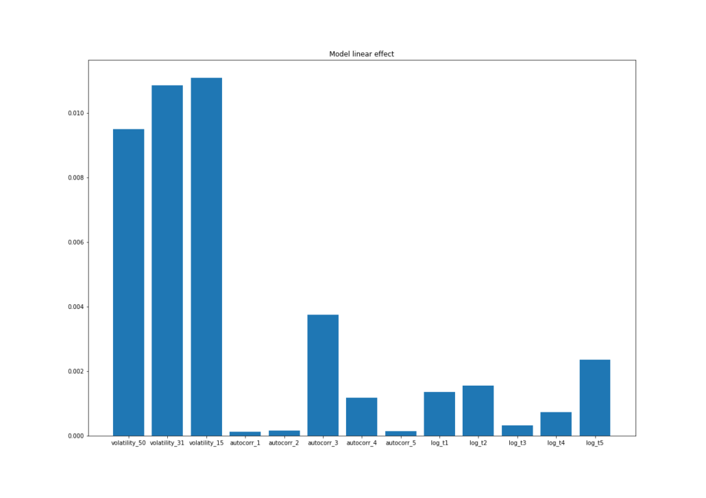
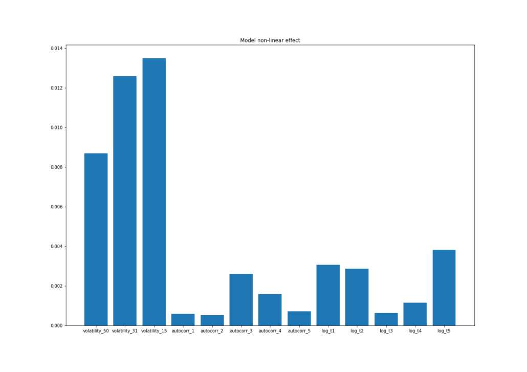
What we can see from all the feature importance plots that the volatility features provide the model with the most value. We would like to use the Fingerprints algorithm to generate more insights about model predictions.

clf_fingerpint = ClassificationModelFingerprint()
clf.fit(X_train, y_train)

feature_combinations = [('volatility_50', 'volatility_15'), ('volatility_50', 'autocorr_4'), 
                       ('autocorr_1', 'autocorr_4'), ('autocorr_4', 'volatility_15'), ('volatility_50', 'log_t4'),
                       ('volatility_31', ('autocorr_4'))]

clf_fingerpint.fit(clf, X_train, num_values=50, pairwise_combinations=feature_combinations)


# Plot linear effect
plt.figure(figsize=(17, 12))
plt.title('Model linear effect')
plt.bar(*zip(*clf_fingerpint.linear_effect['raw'].items()))
plt.savefig('linear.png')

# Plot non-linear effect
plt.figure(figsize=(17, 12))
plt.title('Model non-linear effect')
plt.bar(*zip(*clf_fingerpint.non_linear_effect['raw'].items()))
plt.savefig('non_linear.png')

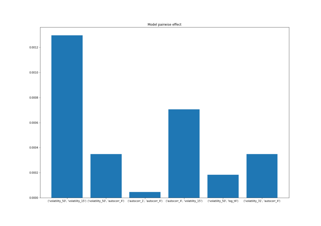
# Plot pairwise effect
plt.figure(figsize=(17, 12))
plt.title('Model pairwise effect')
plt.bar(*zip(*clf_fingerpint.pair_wise_effect['raw'].items()))
plt.savefig('pairwise.png')

What we can see from Fingerprints algorithm is a strong linear, non-linear and pairwise effect for volatility features. It also coincides with MDI, MDA and SFI results. What can a researcher conclude from this? Volatility is an important factor used to determine the probability of success of SMA crossover trend system.

We may also conclude that other features are not that informative for our model. In this case, the next research step would be to concentrate more on volatility type of features and extract more information from them. Try estimating the entropy of volatility values, generate volatility with bigger look-back periods, take the difference between volatility estimates and so on.

Conclusion

In this post we have shown how the mlfinlab package is used to perform feature importance analysis using MDI, MDA, SFI and the Model Fingerprints algorithm. The approach described above is just one of many ways to interpret a machine learning model. One can also use Shapley values, and the LIME algorithm to get the intuition behind the model’s predictions.