Machine Learning Trading Essentials (Part 2): Fractionally differentiated features, Filtering, and Labelling

by Michael Meyer and Masimba Gonah

Introduction

Welcome back, fellow traders and machine learning enthusiasts! We hope you’ve been enjoying our journey towards building a successful machine learning trading strategy. If you missed Part 1 of our series, don’t fret – you can always catch up on our exploration of various financial data structures, such as dollar bars. In this post, we’ll continue to investigate key concepts related to using machine learning for trading, with a focus on techniques that can aid in the model development process.

At its core, machine learning is all about using data to make predictions and decisions. In the context of trading, this means analyzing vast amounts of financial data to identify patterns and generate profitable trading strategies. However, developing a successful trading strategy is no easy feat — it requires a deep understanding of financial markets, statistical analysis, and the application of various machine learning techniques.

To tackle this challenge, we’ll be exploring a range of techniques that can help us develop a robust and profitable machine learning trading strategy. From fractionally differentiated features, to CUSUM filters and triple-barrier labeling, we’ll be diving into the nitty-gritty details of each technique and how it can be applied in practice.

So buckle up and get ready for an exciting journey into the world of machine learning for trading. Let’s get started!

Let’s quickly give an overview of the techniques that we will investigate in this post:

1. Fractionally differentiated features: In finance, time-series data often exhibits long-term dependence or memory, which can result in spurious correlations and suboptimal trading strategies. Fractionally differentiated features aim to alleviate this issue by applying fractional differentiation to the time series data, which can help to remove the long-term dependence and improve the statistical properties of the data.
2. CUSUM filter: CUSUM stands for “cumulative sum.” A CUSUM filter is a statistical quality control technique that can be used to detect changes in the mean of a time series. In the context of trading, CUSUM filters can be applied to identify periods of abnormal returns, which can be used to adjust trading strategies accordingly.
3. Triple-barrier labelling: This technique involves defining three barriers around a price point to create an “event.” For example, we can define a “bullish” event as when the price increases by a certain percentage within a certain time frame, and a “bearish” event as when the price decreases by a certain percentage within a certain time frame. Triple-barrier labelling is often used in finance to create labeled data for supervised learning models.

Fractionally differentiated features

One of the biggest challenges of quantitative analysis in finance is that price time series have trends (another way of saying the mean of the time-series is non-constant). This makes the time series non-stationary. Non-stationary time series are difficult to work with when we want to do inferential analysis based on the variance of returns, or probability of loss (to name a few examples).

When is a time series considered stationary though? Stationarity refers to a property of a time series where its statistical properties such as mean, variance, and autocorrelation remain constant over time. More formally, a time series is said to be stationary if its probability distribution is the same at every point in time.

Stationarity is an important property because it simplifies the statistical analysis of a time series. Specifically, if a time series is stationary, it allows us to make certain assumptions about the behavior of the data that would not be valid if the data were non-stationary. For example, we can use standard statistical techniques such as autoregressive models, moving average models, and ARIMA models to make predictions and forecast future values of a stationary time series.

In contrast, if a time series is non-stationary, its statistical properties change over time, making it more difficult to model and predict. For example, a non-stationary time series may have a trend or seasonal component that causes the mean and variance to change over time. As a result, we need to use more complex modeling techniques such as differencing or detrending to remove these components and make the data stationary before we can use traditional statistical techniques for forecasting and analysis.

A simple graphical representation is given below of the difference between a stationary and a non-stationary series:

In addition to the simpler statistical analysis, many supervised learning algorithms have the underlying assumption that the data is itself stationary. Specifically, in supervised learning, one needs to map hitherto unseen observations to a set of labelled examples and determine the label of the new observation.

According to Prof. Marcos Lopez de Prado: “If the features are not stationary we cannot map the new observation to a large number of known examples”. Making time series stationary often requires stationary data transformations, such as integer differentiation. These transformations however, remove memory from the series.

The concept of “memory” refers to the idea that past values of a time series can have an effect on its future values. Specifically, a time series is said to have memory if the value of the series at time \(t\) is dependent on its past values at times \(t-1, t-2, t-3\), and so on. The presence of memory in a time series can have important implications for modeling and forecasting.

The presence and strength of memory in a time series can be quantified using autocorrelation and partial autocorrelation functions. Autocorrelation measures the correlation between a time series and its lagged values at different time lags, while partial autocorrelation measures the correlation between the series and its lagged values after removing the effects of intervening lags. The presence of significant autocorrelation or partial autocorrelation at certain lags indicates the presence of memory in the time series.

Fractional differentiation is a technique that can be used in an attempt to remove long-term dependencies in a time series, which can potentially make the series more stationary while still preserving memory. This is achieved by taking the fractional difference of the series, which involves taking the difference between the values of the series at different lags, with a non-integer number of lags. The order of differentiation is chosen based on the degree of non-stationarity in the series, and it can be estimated using statistical techniques such as the Hurst exponent or the autocorrelation function. The method is somewhat complicated and a full explanation of this method can be found in this article.

The order of differentiation in fractional differencing is typically denoted by \(d\), which can be a non-integer value. The value of \(d\) determines the degree of smoothness or roughness in the resulting series.

If the input series:

• is already stationary, then  \(d=0\).
• contains a unit root, then  \(d<1\).
• exhibits explosive behaviour (like in a bubble), then  \(d>1\).

A particularly interesting case is  \(d \ll 1\), which occurs when the original series is “mildly non-stationary”. In this case, although differentiation is needed, a full integer differentiation removes excessive memory (and thus predictive power). We want to use a \(d\) that preserves maximal memory while making the series stationary. To this end, we plot the Augment Dicker Fuller (ADF) statistics for different values of \(d\) to see at which point the series becomes stationary, and also the correlation to the original series (\(d = 0\)) which quantifies the amount of memory that we preserve.

For this, we will again rely on MLFinLab, our quantitative finance Python package, to leverage these techniques. The code presented here builds on Part 1, where we previously processed the data in QuantConnect and generated the dollar bars.

To begin, we calculate the p-value of the original series, which turns out to be 0.77. This is done using the statsmodels library and an ADF test as can be seen in the code below. This value leads us to reject the null hypothesis that the series is stationary, indicating that it is non-stationary. Consequently, we need to apply a transformation to the series to make it stationary before proceeding further. To achieve this we first plot the ADF test statistics for different values of \(d=0\) ranging from 0 to 1 to see for which values of \(d=0\) the differentiated series is stationary. We do this by calling the fracdiff module from MLFinLab and using the plot_min_ffd() function, and passing in the normal series:

from mlfinlab.features import fracdiff
from statsmodels.tsa.stattools import adfuller

# Creating an ADF test
calc_p_value = lambda s: adfuller(s, autolag='AIC')[1]

dollar_series = dollar_bars['close']
dollar_series.index = dollar_bars['date_time']

# Test if series is stationary
calc_p_value(dollar_series)

# plot the graph
fracdiff.plot_min_ffd(dollar_series)

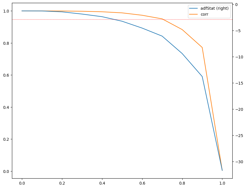
The graph displays several key measures used to analyze the input series after applying a differentiation transformation. The left y-axis shows the correlation between the original series (\(d=0\)) and the differentiated series at various d values, while the right y-axis displays the Augmented Dickey-Fuller (ADF) statistic computed on the downsampled daily frequency data. The x-axis represents the \(d\) value used to generate the differentiated series for the ADF statistic.

The horizontal dotted line represents the critical value of the ADF test at a 95% confidence level. By analyzing where the ADF statistic crosses this threshold, we can determine the minimum \(d\) value that achieves stationarity.

Furthermore, the correlation coefficient at a given \(d\) value indicates the amount of memory given up to achieve stationarity. The higher the correlation coefficient, the less memory was sacrificed to achieve stationarity. Therefore we want to select a \(d\) with the highest correlation while simultaneously achieving stationarity.

In this graph, we observe that the value cut-offs occur just before \(d = 0.5\). Therefore, we set the \(d\) value to 0.5 to ensure that we obtain a stationary series:

fd_series_dollar = fracdiff.frac_diff_ffd(dollar_series, diff_amt=0.5).dropna()
print(calc_p_value(dollar_series))
fd_series_dollar.plot()

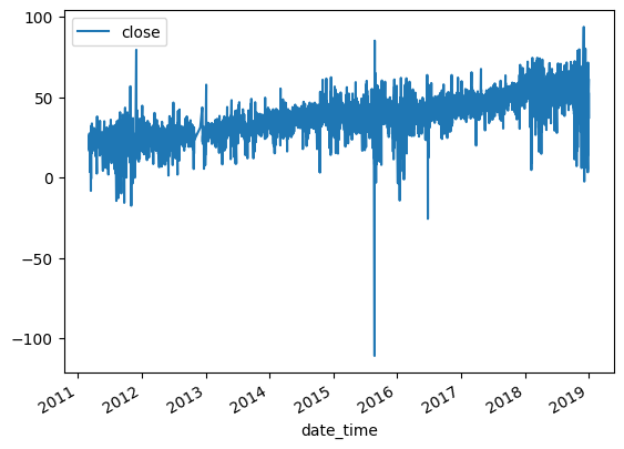
After applying fractional differencing to the time series, we find that the resulting series was stationary based on the p-value obtained from an Augmented Dickey-Fuller test. However, when we plot the series, we observe that there was still some residual drift in the data. This means that the series is not completely stationary yet, and still exhibits some trends over time.

When applying a moving window to differentiate a time series, we obtain a differentiated series that has a tendency to drift over time due to the added weights of the expanding window. In order to eliminate this drift, we can apply a threshold to drop weights that fall below a certain threshold. This helps to stabilize the differentiated series and reduce the impact of the expanding window.

The benefit of using a fixed-width window is that the same vector of weights is used across all estimates of the differentiated series, resulting in a more stable and driftless blend of signal plus noise. “Noise” refers to the random fluctuations in the data that cannot be explained by the underlying trend or seasonal patterns. By removing the impact of the expanding window, we can obtain a stationary time series that has a well-defined statistical properties. The distribution is no longer Gaussian because of the skewness and excess kurtosis that comes with memory, but the stationarity property is achieved.

fd_series_dollar = fracdiff.frac_diff_ffd(dollar_series, diff_amt=0.5,thresh=0.000001).dropna()
print(p_val(fd_series_dollar))
fd_series_dollar.plot()

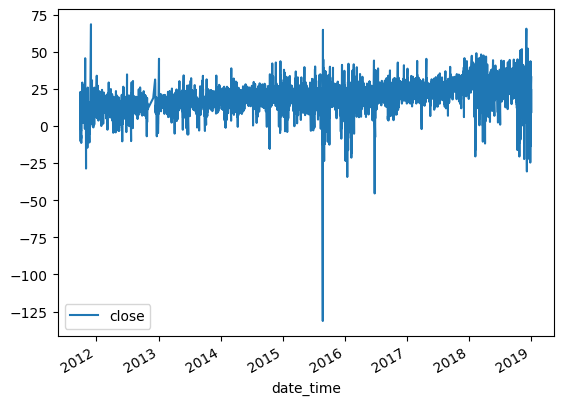
In this modified scenario, we observe almost no drift, and the p-value is 1.10e-18, indicating that the series is statistically stationary and has a maximum memory representation. With this stationary series, we can use it as a feature in our machine learning model. It’s worth noting that fractional differencing can be applied not only to returns but also to any other time series data that you may want to add as a feature in your model.

Filtering for events

After having examined methods to render a time series stationary while retaining maximal information, we will now turn our focus to discovering a systematic approach for identifying events that constitute actions, such as making a trade. Filters are used to filter events based on some kind of trigger. For example, a structural break filter can be used to filter events where a structural break occurs. A structural break is a significant shift or change in the underlying properties or parameters of a time series that affects its behavior or statistical properties. This can occur due to a wide range of factors, such as changes in economic policy, shifts in market conditions, or sudden changes in a system or process that generates the data. In Triple-Barrier labeling, this filtered event is then used to measure the return from the event to some event horizon, say a day.

Rather than attempting to label every trading day, researchers should concentrate on predicting how markets respond to specific events, including their movements before, during, and after such occurrences. These events can then serve as inputs for a machine learning model. The fundamental belief is that forecasting market behavior in response to specific events is more productive than trying to label each trading day.

The CUSUM filter is a statistical quality control method that is commonly used to monitor changes in the mean value of a measured quantity over time. The filter is designed to detect shifts in the mean value of the quantity away from a target value.

In the context of sampling a bar, the CUSUM filter can be used to identify a sequence of upside or downside divergences from a reset level zero. The term “bar” typically refers to a discrete unit of time, such as a day or an hour, depending on the context of the application. In this case, the CUSUM filter is used to monitor the mean value of the measured quantity within each bar.

To implement the CUSUM filter, we first set a threshold value that represents the maximum deviation from the target mean that we are willing to tolerate. The filter then computes the cumulative sum of the differences between the actual mean value and the target value for each bar. If the cumulative sum exceeds the threshold, it indicates that there has been a significant shift in the mean value of the quantity. Luckily for us, this is already implemented in our MLFinlab package, and can be applied using only one line of code!

At this point, we would “sample a bar” to determine whether the deviation from the target mean is significant. Sampling a bar refers to examining the data for the current bar to determine whether the deviation from the target mean is large enough to warrant further investigation. The time interval between bars will depend on the specific application.

One of the practical benefits of using CUSUM filters is that they avoid triggering multiple events when a time series approaches a threshold level, which can be a problem with other market signals like Bollinger Bands. Unlike Bollinger Bands, however, which can generate multiple signals when a series hovers around a threshold level. CUSUM filters require a full run of a set length threshold for a series to trigger an event. This makes the signals generated by CUSUM filters more reliable and easier to interpret than other market signals.

Once we have obtained this subset of event-driven bars, we will let the ML algorithm determine whether the occurrence of such events constitutes an action .

Here we use a threshold 0.01 to trigger an event. This could also be on a volatility estimate or a series of volatility estimates at each point in time.

With MLFinLab this is straightforward to calculate as the code shows below. The events are then returned which cross the threshold.

events = filters.cusum_filter(dollar_series, threshold=0.01)

# create a boolean mask for observations from 2011
mask = events.year == 2011

# select observations from 2011 using the boolean mask
dt_index_2011 = events[mask]

plt.figure(figsize=(16,12))
ax = df['2011'].plot()
ax.scatter(dt_index_2011 , df.loc[dt_index_2011 ], color='red')
plt.title("CUSUM filtered events")
plt.show()

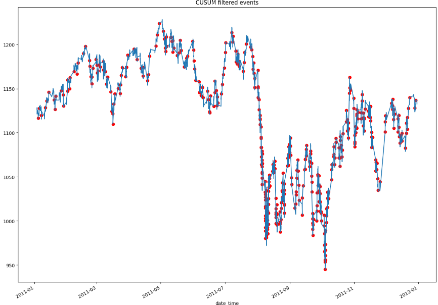
The graph above displays all of the CUSUM filtered events that will be used to train the ML model. It is important to note that the threshold value used to generate these events plays a critical role in determining the number and type of events that are captured. From a practical standpoint, selecting a higher threshold will result in more extreme events being captured, which may contain valuable information for the model. However, if we only capture extreme events there will be fewer events overall to train the ML model on, which could impact the model’s accuracy and robustness. Conversely, selecting a lower threshold will result in more events being captured, but they may be less informative and have less predictive power. Finding the optimal threshold value is often a balancing act between capturing valuable information and having a sufficient number of events to train the ML model effectively.

Labelling

Next we need to label the observations that we use as the target variable in a supervised learning algorithm. We will use the triple-barrier method for this, though there are many other ways to label a return.

The idea behind the triple-barrier method is that we have three barriers: an upper barrier, a lower barrier, and a vertical barrier. The upper barrier represents the threshold an observation’s return needs to reach in order to be considered a buying opportunity (a label of 1), the lower barrier represents the threshold an observation’s return needs to reach in order to be considered a selling opportunity (a label of -1), and the vertical barrier represents the amount of time an observation has to reach its given return in either direction before it is given a label of 0. This concept can be better understood visually and is shown in the figure below taken from Advances in Financial Machine Learning

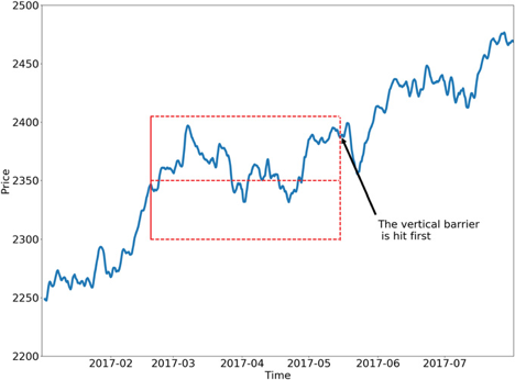
One of the major faults with the fixed-time horizon method is that observations are given a label with respect to a certain threshold after a fixed amount of time regardless of their respective volatilities. In other words, the expected returns of every observation are treated equally regardless of the associated risk. The triple-barrier method tackles this issue by dynamically setting the upper and lower barriers for each observation based on their given volatilities. The dynamic approach ensures that it takes into account the current estimated volatility of the assets it is applied to.

In our case, we set the vertical barrier to 1-day and the profit-take and stop-loss levels at 1% based on the volatility. This, again, should be decided on based on the strategy that you had in mind.

# Compute daily volatility
daily_vol = volatility.get_daily_vol(dollar_series)

# Compute vertical barriers
vertical_barriers = labeling.add_vertical_barrier(t_events=events, close=dollar_series, num_days=1)

# Triple barrier
pt_sl = [1, 1]
min_ret = 0.0005
triple_barrier_events = labeling.get_events(close=dollar_series,
                                            t_events=events,
                                            pt_sl=pt_sl,
                                            target=daily_vol,
                                            min_ret=min_ret,
                                            num_threads=2,
                                            vertical_barrier_times=vertical_barriers)

labels = labeling.get_bins(triple_barrier_events, dollar_series)
print(labels['bin'].value_counts())

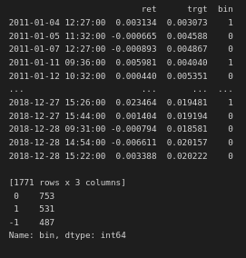
Here we see that we have 1771 observations, with 531 we should go long, 487 short, and 753 we should not make a trade. Using this dataset, we can train a supervised ML model to predict these three classes.

As an additional step , we can take a look at the average sample uniqueness from our new dataset that was labelled by the triple barrier method. Some of the labels may overlap (concurrent labels), leading to sample dependency. To remedy this we can weight an observation based on its given return as well as it’s average uniqueness.

Conclusion

In conclusion, we have taken a look at various ways to process our data so that it can be used in a ML setting. There are many variations on the different techniques and how to use them, but the principles remain the same. The techniques are agnostic to the asset traded and could be applied universally. Next, we will decide on a strategy that we want to test, and decide on useful features, that can hopefully lead to a profitable strategy!