Copula for Pairs Trading: A Unified Overview of Common Strategies
by Hansen Pei
Join the Reading Group and Community: Stay up to date with the latest developments in Financial Machine Learning!
This is the third article of the copula-based statistical arbitrage series. You can read the previous two articles:
Introduction
Systematic approaches of pairs trading gained popularity from the mid-1980s. Gatev et al (2006) examined the profitability of a distance-based strategy on normalized prices. Cointegration is another common strategy incorporated approach as discussed in [Vidyamurthy (2004)]. Both methods are tied to the idea of a mean-reverting bet, and the trading signals are generated from the spread: when the spread widens, it is expected to narrow, and when it does happen the trader pockets the profit.
We have previously talked about several advantages from copula-based models in Copula for Pairs Trading: A Detailed, But Practical Introduction, and as a tool it analyzes the dependence structure among several random variables (For pairs trading it is just 2 random variables). We quickly summarize it here:
- Non-linear relations in tail moves of stocks are naturally captured by copula models. This is often where the buy-low-and-sell-high opportunities arise.
- Copula works with quantiles data, and thus greatly simplifies the workflow by bypassing analyzing idiosyncratic marginal distributions.
Apart from those two relatively known advantages, it has another interesting feature specifically for creating trading strategies: the signal is not generated from the spread but individually from the two legs. Therefore a trader can use different methods to assemble the signals for creating the final long/short/exit decision and thus create a huge amount of variations under the copula framework to avoid a crowded playground.
One way to understand such a feature is that copula models the relative mispricing from each stock, and the end user’s work is to combine to make use of them. Being a relatively novel approach, there is no hard-and-fast rule here, and a lot of work indeed can be done to further improve those strategies especially from pairs-selection. We have looked through the most well-regarded approaches and their variations, and we found it more meaningful to look at them through a unified perspective. This is a truly vast topic and to make this article manageable, we restrict our discussions to the followings:
- What information does copula provide for trading?
- Common trading strategies, variations, and what are the moving parts?
- Common pairs selection methods and what is missing.
- Possible ideas for implementation.
Key Idea: Conditional Probability
Suppose C(u1,u2) is a bivariate copula with uniform random variable input u1 and u2 as quantiles from data mapped by their marginal CDFs, the (cumulative) conditional probabilities for each leg is defined as the following:
![]()
Almost all copula-based pairs trading strategies that I am aware of use conditional probabilities as the core. Their values are interpreted as below:
- When
 , then variable 1 is considered undervalued.
 - When
 , then variable 1 is considered overvalued.
Similarly, this relation holds for variable 2 using ![]() . See the picture below for a demonstration:
. See the picture below for a demonstration:
The histogram represents some independent sample draws from a fixed conditional distribution, thus the total frequency sums up to 1. When the conditional cumulative density is less than 0.5, as shown on the left, the value is considered small. Similarly on the right, it is considered a large value.
A few things to keep in mind: First, this quantity is model dependent, which means it will be almost surely different if you use another different copula. Second, to be able to use a copula for calculating returns series, one needs to fit a copula with historical data, and all the above undervalue or overvalue judgment is based on history. Third, for a given data point ![]() , you will get conditional probabilities from each random variable individually. For example, if the input quantile comes from stock prices, then you will get information like “stock 1 is overpriced, given the current stock 2’s price” and “stock 2 is underpriced, given the current stock 1’s price” together. A very important note is that one does not imply another necessarily, and the copula may tell you that both stocks are overvalued/undervalued sometimes. It depends on you how you would like to assemble the information.
, you will get conditional probabilities from each random variable individually. For example, if the input quantile comes from stock prices, then you will get information like “stock 1 is overpriced, given the current stock 2’s price” and “stock 2 is underpriced, given the current stock 1’s price” together. A very important note is that one does not imply another necessarily, and the copula may tell you that both stocks are overvalued/undervalued sometimes. It depends on you how you would like to assemble the information.
Therefore, all the trading strategies utilizing conditional probabilities can be unified under the following framework. In ArbitrageLab we provided the most commonly used ones that we will discuss for the next few sections, and a few places you can tweak the logic to formulate your strategy.
Thus, the possible moving parts are clear:
- What data to use? Prices or returns?
- How to generate relative mispricing information of stocks from a copula?
- What logic to use to assemble information from the two legs?
LEARN MORE ABOUT PAIRS TRADING STRATEGIES WITH “THE DEFINITIVE GUIDE TO PAIRS TRADING”
Strategy 1: Simple Thresholds on Prices
This is proposed in [Liew et al. 2013] [Botha et al. 2013].
Strategy
This strategy is relatively easy to understand and implement since it works directly with the pair’s prices series using the conditional probability thresholds: Suppose we define an upper threshold bup (e.g. 0.95) and a lower threshold blo (e.g. 0.05), then the logic goes as follows as described in the literature:
- Opening rules:
-
- If
 AND
AND  , then stock 1 is undervalued, and stock 2 is overvalued. Hence we long the spread. (1 in position)
 - If
 AND
AND  , then stock 2 is undervalued, and stock 1 is overvalued. Hence we short the spread. (-1 in position)
- If
- Exit rule:
-
- If BOTH/EITHER conditional probabilities cross the boundary of 0.5, then we exit the position, as we consider the position no longer valid. (0 in position).
Here the spread can come from the hedge ratio using the training data. For example, you can run a simple OLS or use something fancier like the Johansen cointegration test and pick their eigenvectors. Alternatively, you may run a dollar-neutral strategy, which is also quite popular to pair with copula-based methods.
This strategy also works with normalized prices or log prices and will produce an identically fitted copula, since copula uses quantiles data. Any strictly monotone transformation using an increasing function on the marginal data will thus yield identical results.
For ambiguities, the following situations are not specified:
- When there is an open signal and an exit signal.
- When there is an open signal and currently there is a position.
- When there is a long and short signal together.
One can adjust the logic and specify ambiguities to see what happens. Often the change of fundamental logic for signal generation greatly influences the performance of the strategy, and wrong combinations can drive a promising strategy unprofitable. The ambiguities are less influential overall but they still should be specified for a working strategy both for interpretability and preventing unexpected actions.
Comments
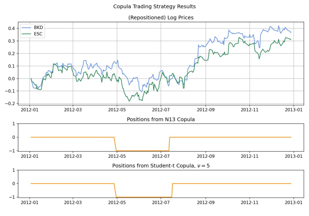
Based on our tests, we found using AND for opening, OR for exiting on average captures better trading opportunities and exits on time. This strategy is also pretty robust: using a different copula with similar fit scores usually leads to almost identical positions and P&L. However we still have a few concerns, regarding using prices series as input:
- Prices of stocks are in general not stationary and since copula uses quantiles data, if a stock has an upward drift then the model will be broken after some time.
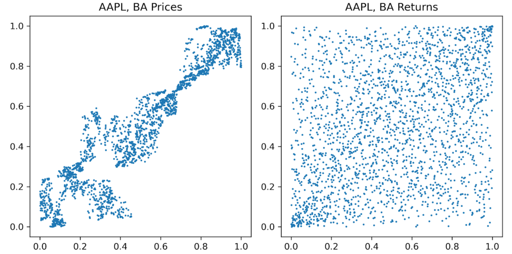
- Copula assumes the input data to be independent draws from two random variables with fixed distributions, and a stock price time series definitely does not satisfy such an assumption. Instead, stock prices have term structures and they tend to aggregate in their Q-Q plot. Such a structure may not be readily described by commonly used copulas and is subject to overfitting even if someone can find a copula on the face that fits.
The first concern can somewhat be mitigated using simple methods. For example, when selecting pairs, use the Hurst exponent to filter all the non-stationary pairs; or update the training set often to keep up with the newest price. But the second concern cannot be fixed as long as we are not incorporating time-varying copula models, which is not under our current concern and is a serious topic that deserves its own discussion.
Instead, working with returns data can by large resolve the above issues: returns are in general stationary around 0, and they are much closer to the i.i.d. assumption imposed by copulas compared to prices. But in general, stocks are not traded directly on returns but prices, so how can we engineer a strategy that is based on returns?
Strategy 2: Cumulative Mispricing Index on Returns
Working with returns is more common in literature for copula-based methods, and this is a building block for other more complicated multi-pairs trading strategies. See [Xie et al. 2014] [Stübinger et al. 2016] [Rad et al. 2016] [da Silva et al. 2017].
Concepts
To use returns to generate trading signals, one eventually needs to translate the information from overvalued/undervalued returns to mispricing.
Mispricing Index (MPI)
MPI is defined as the conditional probability of returns, i.e.,
![]()
![]()
for stocks ![]() with returns random variable at day
with returns random variable at day ![]() :
: ![]() and specific returns value at day
and specific returns value at day ![]() :
: ![]() . The MPIs determine conditionally if the return on that day is over or under the average. Note that so far only one day’s return information contributes, and naturally we want to cumulatively add a few days of MPIs up to gauge whether each stock is mispriced. This idea is not at all new, for example, when log-prices can be constructed from adding up log-returns.
. The MPIs determine conditionally if the return on that day is over or under the average. Note that so far only one day’s return information contributes, and naturally we want to cumulatively add a few days of MPIs up to gauge whether each stock is mispriced. This idea is not at all new, for example, when log-prices can be constructed from adding up log-returns.
Cumulative Mispricing Index (CMPI) / Flags
Well, we are almost there. For ease of analysis, we also need to subtract the average 0.5 before adding up the daily MPIs, because they are probabilities. It is easier to think about a quantity is overvalued/undervalued if the indicator is greater/lesser than 0. Therefore we introduce the cumulative mispricing index (CMPI, in some literature and in our module it is also called Flags) series as below
![]()
![]()
If ![]() then stock X is overvalued; if
then stock X is overvalued; if ![]() then stock X is undervalued. Same for
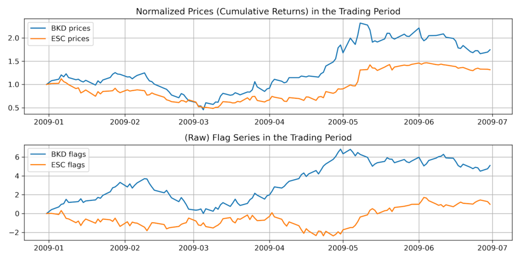
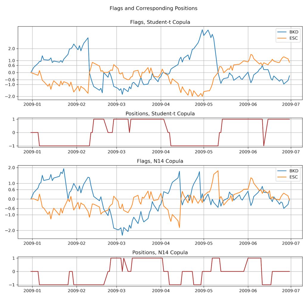
then stock X is undervalued. Same for ![]() . We plot the raw flags series as below and they look quite similar to cumulative log-returns (just another way of saying log-prices!) from their price series, which is what they were designed to do: to reflect price information from returns.
. We plot the raw flags series as below and they look quite similar to cumulative log-returns (just another way of saying log-prices!) from their price series, which is what they were designed to do: to reflect price information from returns.
Trading Logic
A strategy under the dollar-neutral scheme is worded as follows:
- Opening rules: (
 for example)
-
- When
 reaches
  , short
  and buy
  in equal amounts. (-1 Position)
 - When
 reaches
  , short
  and buy
  in equal amounts. (1 Position)
 - When
 reaches
  , short
  and buy
  in equal amounts. (1 Position)
 - When
 reaches
  , short
  and buy
  in equal amounts. (-1 Position)
- When
- Exiting rules: (
 for example)
-
- If trades are opened based on
 , then they are closed if
  returns to 0 or reaches the stop-loss position
  or
or  .
. - If trades are opened based on
 , then they are closed if
  returns to 0 or reaches the stop-loss position
  or
or  .
.
- If trades are opened based on
- After trades are closed, both
 and
and  are reset to 0.
For ambiguities we have the following:
- When
 reaches
  (or
(or  ) and
) and  reaches
  (or
(or  ) together.
 - When in a long(or short) position, receives a short(or long) trigger.
- When receiving an opening and exiting signal together.
- When the position was open based on
 (or
(or  ),
),  (or
(or  ) reaches
  or
or  .
.
The ambiguity cases occur much more often than the previous strategy and are a fundamental issue for this approach, since the mispricing info is generated from each stock. When assembling the information, conflicting signals should be regarded as normality, not outliers. We will discuss more issues in the comment section below.
Comments
Logic
This strategy overall is way too sensitive. Using the end-of-day data, it is not uncommon to see 6 to 8 position changes in a month. This comes from how the signals are assembled. Looking at the strategy above it essentially uses an OR logic for opening: when stock X OR Y suggests an opening, then the strategy opens a position. For closing, it also uses an OR logic. Another variable is whether we reset the CMPIs to 0. In a nutshell:
- Opening logic: AND, OR
- Exiting logic: AND, OR
- Whether reset: True, False
That is 8 possible combinations! Those choices are built-in for the copula module in ArbitrageLab. Just be aware of the logic that, tracking which stock opened a position only makes sense for the OR-OR open-close logic combination. For all the other three choices, it’s sufficient to directly compare the CMPIs to thresholds. Not so surprisingly, to tune down the sensitivity you can change AND to OR.
Variation by Rad et al (2016)
Rad et al (2016) suggested using AND for opening, OR for exiting, and no reset. Then they did a thorough analysis by comparing this copula strategy variation with distance and cointegration methods. It is an excellent paper that sheds insight on the performance characteristics and I think all the people interested in copula methods should read it. Here are two major results:
- The performance of the copula approach is similar to the more traditional distance and cointegration methods given that the pairs do converge. Overall the copula approach has lower returns because non-convergent pairs drag the performance.
- The copula method has better performance during market downturns across all the pairs.
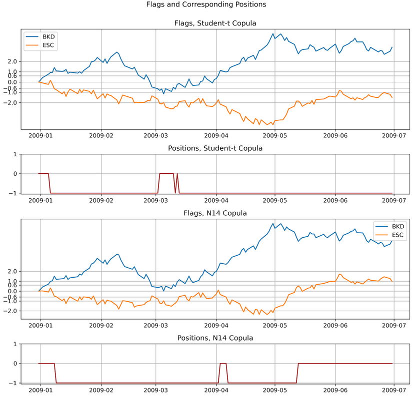
(Moreover, in our research, we found that this variation tends to capture the opening opportunities well, however does not exit at the right time sometimes, which brings down the performance.) We can see that the performance suffers mostly from non-convergent pairs. If the pairs are well-chosen then the copula method will enjoy a similar performance with distance and cointegration method while suffering much less from bear markets. This is no surprise since tail co-moves are baked-in for copula models. For the convergence issue, now let’s look at the two CMPI series generated from the stocks pair:
First, the CMPIs are highly model-dependent. Even using copulas with similar fit scores will lead to possibly very different looking CMPIs and positions are taken based on CMPIs. Secondly, this type of strategy regardless of the logic combinations is betting on the mean-reversion of CMPIs, but they behave more like martingales. Moreover, the commonly used pairs selection methods such as Spearman’s rho, or Euclidean distance do not reflect this key mean-reverting requirement for the CMPI series, also the copula’s prices spread do not necessarily need to be mean-reverting for the copula strategy to be profitable.
Quick Pairs Selection
The commonly used methods are Euclidean distance (![]() -norm on normalized prices, though other P-norms are also reasonable, especially because stocks spread rarely stays at the same value for an extended time that could invalidate large P values if it ever happened.), Kendall’s tau and Spearman’s rho. The rank-based methods offer some protection against extreme values natively, and they are more closely tied to how copulas are fitted.
-norm on normalized prices, though other P-norms are also reasonable, especially because stocks spread rarely stays at the same value for an extended time that could invalidate large P values if it ever happened.), Kendall’s tau and Spearman’s rho. The rank-based methods offer some protection against extreme values natively, and they are more closely tied to how copulas are fitted.
In [Stübinger et al. 2016], other quick and seemingly promising approaches are proposed as well, such as geometric distance to the diagonal on Q-Q plot, and a ![]() measure of independence (thus dependence).
measure of independence (thus dependence).
Comparisons Among the Methods
In general, Kendall’s tau and Spearman’s rho both use quantile data, will rank and select their pairs similarly, though Kendall’s tau requires more computational time (![]() vs.
vs. ![]() ) and is a tad more stable for outliers.
) and is a tad more stable for outliers.
The higher the value of tau or rho, the more co-moves in their quantiles and vice versa. Also due to using percentile data, they are much more resilient to outliers, as compared to Euclidean distance. Euclidean distance will generally select very different pairs, in comparison. The smaller the Euclidean distance, the more close movements the pair of stocks have.
Here, I ran a mini-test for the three criteria using the 30 stocks in the Dow from 2011-2019 with adjusted closing prices for demonstration (Note: this is just for show of those methods. In reality it is a bad idea to feed 10 years of data to a static model.). The calculation is pretty fast, taking about 1 second using my office laptop, so it is readily scalable.
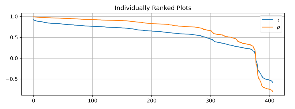
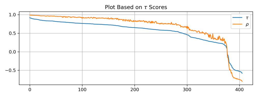
First, let us rank and plot Kendall’s tau and Spearman’s rho values individually. We can see that Kendall’s tau tends to be smaller than Spearman’s rho in absolute value in general.
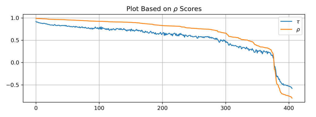
Then let’s verify that they indeed select similar pairs. We do this by plotting Kendall’s tau value using ranks from Spearman’s rho and vice versa.
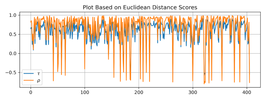
As you can see, Spearman’s rho is slightly less stable than Kendall’s tau, but otherwise, they generate comparable results. The Euclidean distance is very different, here is a plot of rho and tau values using ranks from the Euclidean distance.
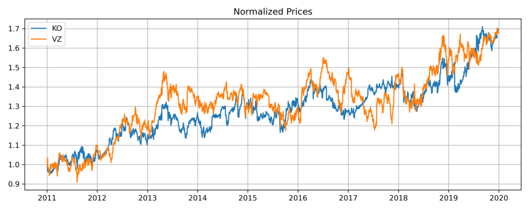
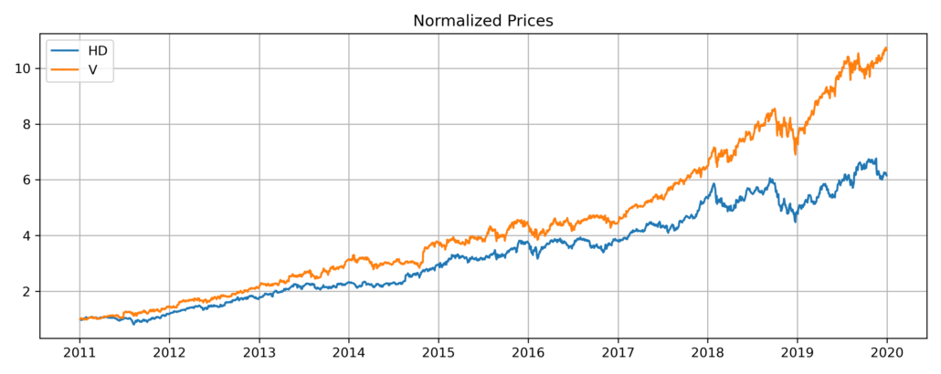
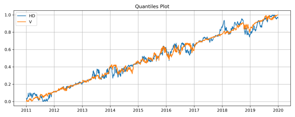
Here are some plots for prices: The KO-VZ pair is the top choice chosen by Euclidean distance, whereas the HD-V pair is chosen by Kendall’s tau.
It might make more sense to look at this pair’s quantile plot on prices instead:
Comments
Users should be aware that the three methods are not specifically made for copulas. When using strategy 2 the desirable property of convergent CMPIs is not captured explicitly by those methods. In [Stübinger et al. 2016], a ![]() independence test criterion demonstrates the best performance for vine copula models, probably from accounting for extreme moves. We, therefore, encourage the reader to test this approach.
independence test criterion demonstrates the best performance for vine copula models, probably from accounting for extreme moves. We, therefore, encourage the reader to test this approach.
Our take overall is that copula methods should come with their own dedicated pairs selecting methods with dedicated goals to match implicit requirements posed by the copula methods. That ![]() method in [Stübinger et al. 2016] may be closer to those goals on average, compared to the three methods defined above. We will dive deeper into this approach in an article for vine copula strategies. Indeed, copula is already a relatively novel approach and some practitioners treat it as a black box. The associated analysis for pairs selection is severely underdeveloped and needs to be taken seriously.
method in [Stübinger et al. 2016] may be closer to those goals on average, compared to the three methods defined above. We will dive deeper into this approach in an article for vine copula strategies. Indeed, copula is already a relatively novel approach and some practitioners treat it as a black box. The associated analysis for pairs selection is severely underdeveloped and needs to be taken seriously.
Other Ideas
Here are a few ideas that are on my shortlist to try out. Some are from other literature that has not been applied to copula in general, some are just thoughts that are easy to implement for empirical analysis. All of the followings can be done with just a few lines of code since the CMPIs values can be directly returned in the module.
- Use Bollinger Band for generating trading signals from each stock: when the CMPIs is greater than the band’s upper bound, then generate a short signal, lesser for a long signal. Then assemble the signal via AND/OR.
- Instead of comparing CMPIs with 0 for long/short/exit, compare the two CMPIs with each other by building a distance strategy based on it. It is natural to think about comparison of performance between the original distance strategy and a distance strategy based on CMPIs.
- Run the CMPIs for pairs selection, and only choose those pairs that have converging CMPIs.
- Mix the prices-based strategies and returns-based strategies, since the former is robust and the latter is sensitive.
- Copulating with alternative data. This is easier when using higher-dimensional copula models for instance in vine copula.
Conclusion
Copula is no panacea for pairs trading. I hope you find it helpful for understanding these strategies after reading through this article. Essentially it is just a mathematical tool that is born to describe the dependence structure among univariate random variables. When applied to generating trading signals there are a lot of moving parts and room for improvising.
The sophistication of copula-based methods still seems somewhat lacking, given that most known methods are just variations of strategy 1 and 2, using simple conditional probabilities. There are also no dedicated copula-based strategies for trading when the tail events happen, given that copula models perform well with tail risks.
We expect further developments and popularity to emerge in this field in the foreseeable future, both in the aspect of strategy complexity (e.g., using more than just the conditional probability for signal generation) and model complexity (e.g., using vine copula for exploiting mispricing in a cohort of stocks).
References
- B Sabino da Silva, F., Ziegelman, F. and Caldeira, J., 2017. Mixed Copula Pairs Trading Strategy on the S&P 500. Flávio and Caldeira, João, Mixed Copula Pairs Trading Strategy on the S&P, 500.
- Liew, R.Q. and Wu, Y., 2013. Pairs trading: A copula approach. Journal of Derivatives & Hedge Funds, 19(1), pp.12-30.
- Patton, A.J., 2012. A review of copula models for economic time series. Journal of Multivariate Analysis, 110, pp.4-18.
- Patton, A.J., 2009. Copula–based models for financial time series. In Handbook of financial time series (pp. 767-785). Springer, Berlin, Heidelberg.
- Rad, H., Low, R.K.Y. and Faff, R., 2016. The profitability of pairs trading strategies: distance, cointegration and copula methods. Quantitative Finance, 16(10), pp.1541-1558.
- Stander, Y., Marais, D. and Botha, I., 2013. Trading strategies with copulas. Journal of Economic and Financial Sciences, 6(1), pp.83-107.
- Stübinger, J., Mangold, B. and Krauss, C., 2018. Statistical arbitrage with vine copulas. Quantitative Finance, 18(11), pp.1831-1849.
- Vidyamurthy, G., 2004. Pairs Trading: quantitative methods and analysis (Vol. 217). John Wiley & Sons.
- Xie, W., Liew, R.Q., Wu, Y. and Zou, X., 2016. Pairs trading with copulas. The Journal of Trading, 11(3), pp.41-52.

