Posts

by Michael Meyer and Masimba Gonah

Introduction

Welcome back, fellow traders and machine learning enthusiasts! We hope you’ve been enjoying our journey towards building a successful machine learning trading strategy. If you missed Part 1 of our series, don’t fret – you can always catch up on our exploration of various financial data structures, such as dollar bars. In this post, we’ll continue to investigate key concepts related to using machine learning for trading, with a focus on techniques that can aid in the model development process.

At its core, machine learning is all about using data to make predictions and decisions. In the context of trading, this means analyzing vast amounts of financial data to identify patterns and generate profitable trading strategies. However, developing a successful trading strategy is no easy feat — it requires a deep understanding of financial markets, statistical analysis, and the application of various machine learning techniques.

To tackle this challenge, we’ll be exploring a range of techniques that can help us develop a robust and profitable machine learning trading strategy. From fractionally differentiated features, to CUSUM filters and triple-barrier labeling, we’ll be diving into the nitty-gritty details of each technique and how it can be applied in practice.

So buckle up and get ready for an exciting journey into the world of machine learning for trading. Let’s get started!

Let’s quickly give an overview of the techniques that we will investigate in this post:

  1. Fractionally differentiated features: In finance, time-series data often exhibits long-term dependence or memory, which can result in spurious correlations and suboptimal trading strategies. Fractionally differentiated features aim to alleviate this issue by applying fractional differentiation to the time series data, which can help to remove the long-term dependence and improve the statistical properties of the data.
  2. CUSUM filter: CUSUM stands for “cumulative sum.” A CUSUM filter is a statistical quality control technique that can be used to detect changes in the mean of a time series. In the context of trading, CUSUM filters can be applied to identify periods of abnormal returns, which can be used to adjust trading strategies accordingly.
  3. Triple-barrier labelling: This technique involves defining three barriers around a price point to create an “event.” For example, we can define a “bullish” event as when the price increases by a certain percentage within a certain time frame, and a “bearish” event as when the price decreases by a certain percentage within a certain time frame. Triple-barrier labelling is often used in finance to create labeled data for supervised learning models.

Fractionally differentiated features

One of the biggest challenges of quantitative analysis in finance is that price time series have trends (another way of saying the mean of the time-series is non-constant). This makes the time series non-stationary. Non-stationary time series are difficult to work with when we want to do inferential analysis based on the variance of returns, or probability of loss (to name a few examples).

When is a time series considered stationary though? Stationarity refers to a property of a time series where its statistical properties such as mean, variance, and autocorrelation remain constant over time. More formally, a time series is said to be stationary if its probability distribution is the same at every point in time.

Stationarity is an important property because it simplifies the statistical analysis of a time series. Specifically, if a time series is stationary, it allows us to make certain assumptions about the behavior of the data that would not be valid if the data were non-stationary. For example, we can use standard statistical techniques such as autoregressive models, moving average models, and ARIMA models to make predictions and forecast future values of a stationary time series.

In contrast, if a time series is non-stationary, its statistical properties change over time, making it more difficult to model and predict. For example, a non-stationary time series may have a trend or seasonal component that causes the mean and variance to change over time. As a result, we need to use more complex modeling techniques such as differencing or detrending to remove these components and make the data stationary before we can use traditional statistical techniques for forecasting and analysis.

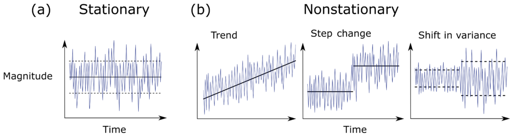
A simple graphical representation is given below of the difference between a stationary and a non-stationary series:

In addition to the simpler statistical analysis, many supervised learning algorithms have the underlying assumption that the data is itself stationary. Specifically, in supervised learning, one needs to map hitherto unseen observations to a set of labelled examples and determine the label of the new observation.

According to Prof. Marcos Lopez de Prado: “If the features are not stationary we cannot map the new observation to a large number of known examples”. Making time series stationary often requires stationary data transformations, such as integer differentiation. These transformations however, remove memory from the series.

The concept of “memory” refers to the idea that past values of a time series can have an effect on its future values. Specifically, a time series is said to have memory if the value of the series at time \(t\) is dependent on its past values at times \(t-1, t-2, t-3\), and so on. The presence of memory in a time series can have important implications for modeling and forecasting.

The presence and strength of memory in a time series can be quantified using autocorrelation and partial autocorrelation functions. Autocorrelation measures the correlation between a time series and its lagged values at different time lags, while partial autocorrelation measures the correlation between the series and its lagged values after removing the effects of intervening lags. The presence of significant autocorrelation or partial autocorrelation at certain lags indicates the presence of memory in the time series.

Fractional differentiation is a technique that can be used in an attempt to remove long-term dependencies in a time series, which can potentially make the series more stationary while still preserving memory. This is achieved by taking the fractional difference of the series, which involves taking the difference between the values of the series at different lags, with a non-integer number of lags. The order of differentiation is chosen based on the degree of non-stationarity in the series, and it can be estimated using statistical techniques such as the Hurst exponent or the autocorrelation function. The method is somewhat complicated and a full explanation of this method can be found in this article.

The order of differentiation in fractional differencing is typically denoted by \(d\), which can be a non-integer value. The value of \(d\) determines the degree of smoothness or roughness in the resulting series.

If the input series:

  • is already stationary, then  \(d=0\).
  • contains a unit root, then  \(d<1\).
  • exhibits explosive behaviour (like in a bubble), then  \(d>1\).

A particularly interesting case is  \(d \ll 1\), which occurs when the original series is “mildly non-stationary”. In this case, although differentiation is needed, a full integer differentiation removes excessive memory (and thus predictive power). We want to use a \(d\) that preserves maximal memory while making the series stationary. To this end, we plot the Augment Dicker Fuller (ADF) statistics for different values of \(d\) to see at which point the series becomes stationary, and also the correlation to the original series (\(d = 0\)) which quantifies the amount of memory that we preserve.

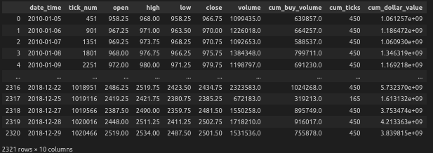
For this, we will again rely on MLFinLab, our quantitative finance Python package, to leverage these techniques. The code presented here builds on Part 1, where we previously processed the data in QuantConnect and generated the dollar bars.

To begin, we calculate the p-value of the original series, which turns out to be 0.77. This is done using the statsmodels library and an ADF test as can be seen in the code below. This value leads us to reject the null hypothesis that the series is stationary, indicating that it is non-stationary. Consequently, we need to apply a transformation to the series to make it stationary before proceeding further. To achieve this we first plot the ADF test statistics for different values of \(d=0\) ranging from 0 to 1 to see for which values of \(d=0\) the differentiated series is stationary. We do this by calling the fracdiff module from MLFinLab and using the plot_min_ffd() function, and passing in the normal series:

from mlfinlab.features import fracdiff
from statsmodels.tsa.stattools import adfuller

# Creating an ADF test
calc_p_value = lambda s: adfuller(s, autolag='AIC')[1]

dollar_series = dollar_bars['close']
dollar_series.index = dollar_bars['date_time']

# Test if series is stationary
calc_p_value(dollar_series)

# plot the graph
fracdiff.plot_min_ffd(dollar_series)

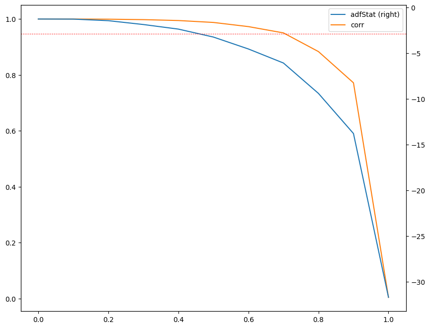
The graph displays several key measures used to analyze the input series after applying a differentiation transformation. The left y-axis shows the correlation between the original series (\(d=0\)) and the differentiated series at various d values, while the right y-axis displays the Augmented Dickey-Fuller (ADF) statistic computed on the downsampled daily frequency data. The x-axis represents the \(d\) value used to generate the differentiated series for the ADF statistic.

The horizontal dotted line represents the critical value of the ADF test at a 95% confidence level. By analyzing where the ADF statistic crosses this threshold, we can determine the minimum \(d\) value that achieves stationarity.

Furthermore, the correlation coefficient at a given \(d\) value indicates the amount of memory given up to achieve stationarity. The higher the correlation coefficient, the less memory was sacrificed to achieve stationarity. Therefore we want to select a \(d\) with the highest correlation while simultaneously achieving stationarity.

In this graph, we observe that the value cut-offs occur just before \(d = 0.5\). Therefore, we set the \(d\) value to 0.5 to ensure that we obtain a stationary series:

fd_series_dollar = fracdiff.frac_diff_ffd(dollar_series, diff_amt=0.5).dropna()
print(calc_p_value(dollar_series))
fd_series_dollar.plot()

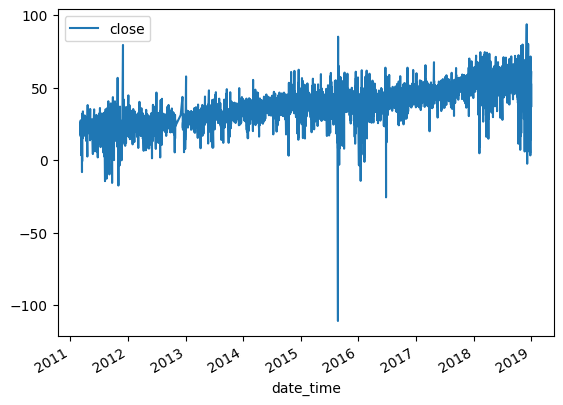
After applying fractional differencing to the time series, we find that the resulting series was stationary based on the p-value obtained from an Augmented Dickey-Fuller test. However, when we plot the series, we observe that there was still some residual drift in the data. This means that the series is not completely stationary yet, and still exhibits some trends over time.

When applying a moving window to differentiate a time series, we obtain a differentiated series that has a tendency to drift over time due to the added weights of the expanding window. In order to eliminate this drift, we can apply a threshold to drop weights that fall below a certain threshold. This helps to stabilize the differentiated series and reduce the impact of the expanding window.

The benefit of using a fixed-width window is that the same vector of weights is used across all estimates of the differentiated series, resulting in a more stable and driftless blend of signal plus noise. “Noise” refers to the random fluctuations in the data that cannot be explained by the underlying trend or seasonal patterns. By removing the impact of the expanding window, we can obtain a stationary time series that has a well-defined statistical properties. The distribution is no longer Gaussian because of the skewness and excess kurtosis that comes with memory, but the stationarity property is achieved.

fd_series_dollar = fracdiff.frac_diff_ffd(dollar_series, diff_amt=0.5,thresh=0.000001).dropna()
print(p_val(fd_series_dollar))
fd_series_dollar.plot()

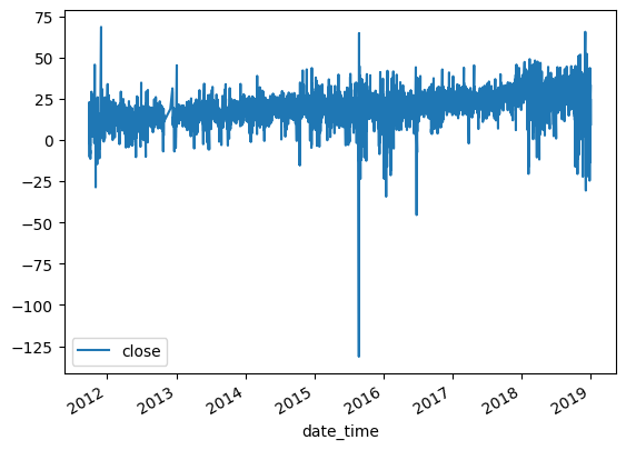
In this modified scenario, we observe almost no drift, and the p-value is 1.10e-18, indicating that the series is statistically stationary and has a maximum memory representation. With this stationary series, we can use it as a feature in our machine learning model. It’s worth noting that fractional differencing can be applied not only to returns but also to any other time series data that you may want to add as a feature in your model.

Filtering for events

After having examined methods to render a time series stationary while retaining maximal information, we will now turn our focus to discovering a systematic approach for identifying events that constitute actions, such as making a trade. Filters are used to filter events based on some kind of trigger. For example, a structural break filter can be used to filter events where a structural break occurs. A structural break is a significant shift or change in the underlying properties or parameters of a time series that affects its behavior or statistical properties. This can occur due to a wide range of factors, such as changes in economic policy, shifts in market conditions, or sudden changes in a system or process that generates the data. In Triple-Barrier labeling, this filtered event is then used to measure the return from the event to some event horizon, say a day.

Rather than attempting to label every trading day, researchers should concentrate on predicting how markets respond to specific events, including their movements before, during, and after such occurrences. These events can then serve as inputs for a machine learning model. The fundamental belief is that forecasting market behavior in response to specific events is more productive than trying to label each trading day.

The CUSUM filter is a statistical quality control method that is commonly used to monitor changes in the mean value of a measured quantity over time. The filter is designed to detect shifts in the mean value of the quantity away from a target value.

In the context of sampling a bar, the CUSUM filter can be used to identify a sequence of upside or downside divergences from a reset level zero. The term “bar” typically refers to a discrete unit of time, such as a day or an hour, depending on the context of the application. In this case, the CUSUM filter is used to monitor the mean value of the measured quantity within each bar.

To implement the CUSUM filter, we first set a threshold value that represents the maximum deviation from the target mean that we are willing to tolerate. The filter then computes the cumulative sum of the differences between the actual mean value and the target value for each bar. If the cumulative sum exceeds the threshold, it indicates that there has been a significant shift in the mean value of the quantity. Luckily for us, this is already implemented in our MLFinlab package, and can be applied using only one line of code!

At this point, we would “sample a bar” to determine whether the deviation from the target mean is significant. Sampling a bar refers to examining the data for the current bar to determine whether the deviation from the target mean is large enough to warrant further investigation. The time interval between bars will depend on the specific application.

One of the practical benefits of using CUSUM filters is that they avoid triggering multiple events when a time series approaches a threshold level, which can be a problem with other market signals like Bollinger Bands. Unlike Bollinger Bands, however, which can generate multiple signals when a series hovers around a threshold level. CUSUM filters require a full run of a set length threshold for a series to trigger an event. This makes the signals generated by CUSUM filters more reliable and easier to interpret than other market signals.

Once we have obtained this subset of event-driven bars, we will let the ML algorithm determine whether the occurrence of such events constitutes an action .

Here we use a threshold 0.01 to trigger an event. This could also be on a volatility estimate or a series of volatility estimates at each point in time.

With MLFinLab this is straightforward to calculate as the code shows below. The events are then returned which cross the threshold.

events = filters.cusum_filter(dollar_series, threshold=0.01)

# create a boolean mask for observations from 2011
mask = events.year == 2011

# select observations from 2011 using the boolean mask
dt_index_2011 = events[mask]

plt.figure(figsize=(16,12))
ax = df['2011'].plot()
ax.scatter(dt_index_2011 , df.loc[dt_index_2011 ], color='red')
plt.title("CUSUM filtered events")
plt.show()

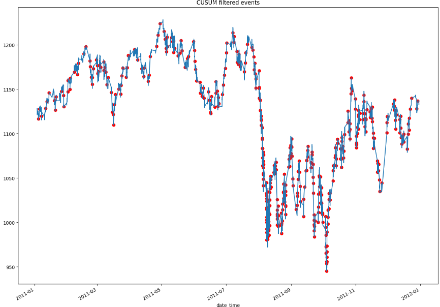
The graph above displays all of the CUSUM filtered events that will be used to train the ML model. It is important to note that the threshold value used to generate these events plays a critical role in determining the number and type of events that are captured. From a practical standpoint, selecting a higher threshold will result in more extreme events being captured, which may contain valuable information for the model. However, if we only capture extreme events there will be fewer events overall to train the ML model on, which could impact the model’s accuracy and robustness. Conversely, selecting a lower threshold will result in more events being captured, but they may be less informative and have less predictive power. Finding the optimal threshold value is often a balancing act between capturing valuable information and having a sufficient number of events to train the ML model effectively.

Labelling

Next we need to label the observations that we use as the target variable in a supervised learning algorithm. We will use the triple-barrier method for this, though there are many other ways to label a return.

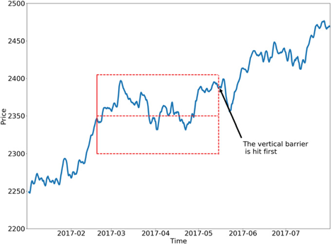
The idea behind the triple-barrier method is that we have three barriers: an upper barrier, a lower barrier, and a vertical barrier. The upper barrier represents the threshold an observation’s return needs to reach in order to be considered a buying opportunity (a label of 1), the lower barrier represents the threshold an observation’s return needs to reach in order to be considered a selling opportunity (a label of -1), and the vertical barrier represents the amount of time an observation has to reach its given return in either direction before it is given a label of 0. This concept can be better understood visually and is shown in the figure below taken from Advances in Financial Machine Learning

One of the major faults with the fixed-time horizon method is that observations are given a label with respect to a certain threshold after a fixed amount of time regardless of their respective volatilities. In other words, the expected returns of every observation are treated equally regardless of the associated risk. The triple-barrier method tackles this issue by dynamically setting the upper and lower barriers for each observation based on their given volatilities. The dynamic approach ensures that it takes into account the current estimated volatility of the assets it is applied to.

In our case, we set the vertical barrier to 1-day and the profit-take and stop-loss levels at 1% based on the volatility. This, again, should be decided on based on the strategy that you had in mind.

# Compute daily volatility
daily_vol = volatility.get_daily_vol(dollar_series)

# Compute vertical barriers
vertical_barriers = labeling.add_vertical_barrier(t_events=events, close=dollar_series, num_days=1)

# Triple barrier
pt_sl = [1, 1]
min_ret = 0.0005
triple_barrier_events = labeling.get_events(close=dollar_series,
                                            t_events=events,
                                            pt_sl=pt_sl,
                                            target=daily_vol,
                                            min_ret=min_ret,
                                            num_threads=2,
                                            vertical_barrier_times=vertical_barriers)

labels = labeling.get_bins(triple_barrier_events, dollar_series)
print(labels['bin'].value_counts())

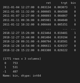
Here we see that we have 1771 observations, with 531 we should go long, 487 short, and 753 we should not make a trade. Using this dataset, we can train a supervised ML model to predict these three classes.

As an additional step , we can take a look at the average sample uniqueness from our new dataset that was labelled by the triple barrier method. Some of the labels may overlap (concurrent labels), leading to sample dependency. To remedy this we can weight an observation based on its given return as well as it’s average uniqueness.

Conclusion

In conclusion, we have taken a look at various ways to process our data so that it can be used in a ML setting. There are many variations on the different techniques and how to use them, but the principles remain the same. The techniques are agnostic to the asset traded and could be applied universally. Next, we will decide on a strategy that we want to test, and decide on useful features, that can hopefully lead to a profitable strategy!

by Michael Meyer and Masimba Gonah

Introduction

Trading in financial markets can be a challenging and complex endeavour, with ever-changing conditions and numerous factors to consider. With markets becoming increasingly competitive all the time, it is a never ending struggle to stay ahead of the curve. Machine learning (ML) has made several advances in recent years, particularly by becoming more accessible. One might think then why not use ML models in markets to challenge more traditional ways of trading? Well the answer is, unfortunately, that it is not so simple.

Financial time series can be challenging to model due to a number of undesirable characteristics that are commonly observed in these series. These characteristics include:

  1. Overfitting: There is a multitude of features that can be used in financial modelling, and it can be difficult to determine which of these features are truly predictive of future behaviour. This can lead to overfitting, where a model performs well on the training data but poorly on the test data (and on real-world data once deployed!).
  2. Non-stationarity: Financial time series often exhibit non-stationarity, which means that the statistical properties of the series change over time. This can make it difficult to model the series using traditional techniques such as linear regression, which assume stationarity in the data.
  3. Heteroscedasticity: Financial time series often display heteroscedasticity, which means that the variance of the series changes over time. This can make it difficult to estimate the true variance of the series and can lead to biased estimates of model parameters.
  4. Autocorrelation: Financial time series often exhibit autocorrelation, which means that the value of the series at one point in time is correlated with the value of itself at another point in time. This can make it difficult to model the series using techniques that assume independence, such as linear regression.

To overcome these challenges, ML models for financial time series should be designed to account for these characteristics, either in the model itself or by transforming the data. For example, we can use ML techniques that are robust to non-stationarity and autocorrelation, by incorporating regularization to reduce overfitting, or by using techniques that account for heteroscedasticity, such as generalized autoregressive conditional heteroscedasticity (GARCH) models.

In this post we’ll take a deep dive into various key aspects of machine learning in trading to overcome some of these challenges. This post is the first in a series. In parts 1 and 2, we will investigate techniques to process data in a suitable manner before feeding it into an ML model. The aim is to get a good understanding of some of the most fundamental concepts, so that an ML model can make sense of the data and extract useful information. Today, we’ll tackle the problem of financial data structures, and see if we can utilize other structures apart from your typical time bars to improve the performance of an ML model.

The concepts are guided by the book Advances in Financial Machine Learning written by Professor Marcos Lopez de Prado . We’ll also introduce you to MLFinLab, our in-house Python package that makes it easy to apply these techniques in your quantitative research and trading.

To get off the ground quickly, we’ll also be partnering with QuantConnect, a platform that offers a wealth of resources for traders of all levels. Whether you’re new to ML or a seasoned pro, this article will give you a step-by-step guide to some of the most fundamental concepts for ML trading.

Overview

To create a robust machine learning trading strategy we’ll follow a set of key steps that help to improve our analysis. To start off, we’ll explore the following concepts:

  1. Financial Data Structures: Instead of relying on traditional time bars, we will investigate dollar bars to structure our financial data. By grouping transactions together based on a fixed dollar amount, we can reduce noise in the data and enhance our ability to identify meaningful patterns.
  2. Fractional differentiation: Applying fractional differentiation can help us transform our financial time series data into a stationary series, which can make it easier to identify trends and signals. By removing drift from the data, we can effectively analyse the underlying patterns, which helps us to make better trading decisions.
  3. CUSUM filter: Filters are used to filter events based on some kind of trigger. We will apply a symmetric CUSUM filter, to detect significant changes in the trend of our financial time series. This filter tracks the cumulative sum of the differences between the expected and observed values, which helps to identify turning points in the trend that may signal buying or selling opportunities.
  4. Triple barrier labelling: Triple barrier labelling allows us to define profit-taking and stop-loss levels for each trade, as well as when not to initiate a trade. By setting upper and lower profit-taking barriers and a stop-loss barrier based on asset volatility, we can automatically exit trades when certain conditions are met.

In part 1 of the article we cover financial data structures.

We will be working in a QuantConnect research node, along with our powerful MLFinLab package. If you’d like to follow along, create a QuantConnect account (there is a free subscription option). You will also need an active subscription to MLFinlab.

Getting started

Let’s dive in!

To start, let’s import the data and transform it into usable format:

# QC construct
qb = QuantBook()

# Specify starting and end times
start_time = datetime(2010, 1, 1)
end_time = datetime(2019, 1, 1 )

# Canonical symbol
es = qb.AddFuture(Futures.Indices.SP500EMini).Symbol

# Continuous future
history = qb.History(es, start_time, end_time, Resolution.Minute, dataNormalizationMode = DataNormalizationMode.BackwardsPanamaCanal)
history = history.droplevel([0, 1], axis=0)  # drop expiry and symbol index, useless in continuous future

data = history
data['date_time'] = data.index
data['price'] = data['close']
data = data[['date_time','price','volume]]

In the code snippet above, we request historical data for S&P 500 E-mini futures contracts. This is a simple process using LEAN, which is QuantConnect’s opensource algorithmic trading engine. The data is freely available on their website to use and you can even download LEAN locally! The contracts are backwards adjusted for the roll, based on the front-month, in order to stitch the contracts together and have a single time series.

We request data from 2010-2018 in minute bars that we will use in our initial analysis. We could’ve also chosen a higher sampling frequency (eg. seconds or even raw ticks), but the computational cost increases significantly as we sample more frequently, so we’ll stick to minute bars.

Financial Data Structures

We will first investigate the different data structures and see what statistical properties they hold, before deciding on an appropriate structure to use.

There are several types of financial data structures, including time bars, tick bars, volume bars, and dollar bars.

  • Time bars are based on a predefined time interval, such as one minute or one hour. Each bar represents the trading activity that occurred within that time interval. For example, a one-minute time bar would show the opening price, closing price, high, and low within one-minute.
  • Tick bars are based on the number of trades that occur. Each bar represents a specified number of trades. For example, a 100-tick bar would show the opening price, closing price, high, and low for the 100 trades that occurred within that bar.
  • Volume bars are based on the total volume of shares traded. Each bar represents a specified volume of shares traded. For example, a 10,000-share volume bar would show the opening price, closing price, high, and low for all trades that occurred until the total volume traded reaches 10,000.
  • Dollar bars are based on the total dollar value of the shares traded. Each bar represents a specified dollar value of shares traded. For example, a $10,000 dollar bar would show the opening price, closing price, high, and low for all trades that occurred until the total dollar value of shares traded reaches $10,000.

Tick bars sample bars more frequently when more trades are executed, while volume bars sample bars more frequently when more volume is traded. While tick bars may be influenced by repetitive or manipulative trades, volume bars bypass this issue by only caring about the total volume traded. However, volume bars may not be effective indicators the value of the asset is fluctuating. To address this, dollar bars can be used instead, which measures the quantity of fiat value exchanged rather than the number of assets exchanged.

To illustrate this concept let’s take a simple example. When someone want to invest they usually decide on a dollar amount to invest, for example investing $10,000 in Apple. The quantity of shares would then be calculated in order to invest that amount. Let’s say you want to invest $10,000 in Apple shares at $100 a share. Then you would buy 100 shares. If the price changes to $200 and you would like to invest the same amount, then you would only buy 50 shares. This examples illustrates that the volume traded is dependant on the price and would not be as consistent as the dollar amount exchanged, which would be the same in both scenarios.

As a result, dollar bars are typically considered more informative than other types of bars, as they provide a more “complete” representation of market activity and can capture periods of high volatility more effectively. A key advantages of dollar bars is that they help to reduce the impact of noise in financial data. In contrast, time-based bars can be affected by periods of low trading activity or market closure, which can result in missing or inaccurate signals. Since dollar bars are constructed based on actual trading activity, they are less susceptible to this type of noise.

But this begs the question: what should the threshold dollar amount exchanged be to form a new dollar bar? When we tried to find an answer, we were surprised to find that very little information exists on this question. Every analysis that we have seen simply uses a constant threshold with no clear explanation to how they derived the threshold amount used.

One suggestion comes Prof. Lopez de Prado who notes that bar size could be adjusted dynamically as a function of the free-floating market capitalisation of a company (in the case of stocks), or the outstanding amount of issued debt (in the case of fixed-income securities). We assume the reason for this is to normalize the amount of money being exchanged by controlling for the total amount of money that could be exchanged, but this is a vague proposition at best and the reason is not quite clear as to why this will improve performance. Sure, the free float market capitalisation is inversely related to volatility, but it is not readily apparent how to make use of this relationship. He also notes that the best statistical properties occur when you sample more or less 50 times a day (meaning you form 50 dollar bars a day), but this is likely an empirical observation.

So to answer this question let’s first think about why we want to use dollar bars. We want to sample on equal buckets of market activity, which is a proxy for equal samples of information. If that is the case, the when should have a sample rate that reflects this activity. Another consideration is the ultimate strategy we want to deploy. If, for example, we have higher frequency trading strategy then we would want to have more granular data and therefore have a higher sampling frequency.

Say we use a constant threshold to form dollar bars. If the fiat value exchanged increase over time (which it most likely will due to inflation for example, or a security becoming more popular to trade) we will on average under sample closer to the start and over sample towards the end over the period we are forming the bars (provided a long enough timespan).

To illustrate this point, let’s look at the volume and dollar amount exchanged over time.

First we will construct time bars using our package MLFinLab. Hudson & Thames has it’s own selectable development environment in QuantConnect, and to use it you only require your API key, which you obtain on purchase. To authenticate MLFinlab on QuantConnect, execute the two lines show below:

import ht_auth
ht_auth.SetToken("YOUR-API-KEY")

Then we can create daily time bars which we will use in our analysis:

# create daily bars
time_bars_daily = time_data_structures.get_time_bars(data, resolution='D', verbose=False)
time_bars_daily.index =  time_bars_daily['date_time']
time_bars_daily

This produces the following output:

Next let’s, take a look at the volume and dollar amounts exchanged over time:

fig, axs = plt.subplots(2, 2, figsize=(12, 12))


monthly_data_volume = time_bars_daily['volume'].resample('M').mean()
monthly_data_dollar = time_bars_daily['cum_dollar_value'].resample('M').mean()

# First subplot: yearly_avg_volume with 12-month rolling window
ax1 = axs[0, 0]
color = '#0C9AAC'
ax1.set_xlabel('Year')
ax1.set_ylabel('Average Volume per day', color=color)
ax1.bar(monthly_data_volume.index, monthly_data_volume.rolling(window=12).mean(), width=30, color=color)
#ax1.tick_params(axis='y', labelcolor=color)
ax1.set_title('Daily Average Volume (12-month window)')

# Second subplot: monthly_data_volume with 1-month rolling window
ax2 = axs[0, 1]
color = '#0C9AAC'
ax2.set_xlabel('Month')
ax2.set_ylabel('Average Volume per day', color=color)
ax2.bar(monthly_data_volume.index, monthly_data_volume.rolling(window=1).mean(), width=30, color=color)
#ax2.tick_params(axis='y', labelcolor=color)
ax2.set_title('Daily Average Volume (1-month window)')

# Third subplot: yearly_avg_dollar with 12-month rolling window
ax3 = axs[1, 0]
color = '#DE612F'
ax3.set_xlabel('Year')
ax3.set_ylabel('Average Dollar amount per day', color=color)
ax3.bar(monthly_data_dollar.index, monthly_data_dollar.rolling(window=12).mean(), width=30, color=color)
#ax3.tick_params(axis='y', labelcolor=color)

ax3.set_title('Daily Average Dollar (12-month window)')

# Fourth subplot: monthly_data_dollar with 1-month rolling window
ax4 = axs[1, 1]
color = '#DE612F'
ax4.set_xlabel('Month')
ax4.set_ylabel('Average Dollar amount per day', color=color)
ax4.bar(monthly_data_dollar.index, monthly_data_dollar.rolling(window=1).mean(), width=30, color=color)
#ax4.tick_params(axis='y', labelcolor=color)
ax4.set_title('Daily Average Dollar (1-month window)')

# Adjust layout and spacing between subplots
plt.tight_layout()

The graphs above displays the average daily average volume and dollar amounts exchanged. The left-hand side uses a rolling window of 12-month and the right-hand side uses rolling window of 1-months to calculate the average daily amount. On a month-to-month basis the amounts fluctuate quite a lot. We can clearly see a trend when using a longer window for both volume and dollar amounts. The volume is decreasing over time while the dollar amount is increasing, which isn’t all that surprising since the price of SPY has increased significantly over the period. Therefore it would make more sense to apply a dynamic threshold.

Another possible reason for using a dynamic threshold is as follows: a known useful feature to use in many strategies is to incorporate the volume traded on a security. If we use dollar bars however, incorporating volume is redundant as the only differential is the price. We can however use the rate of information used to form a bar, for example the time it took to form the bar, or the number of ticks in a bar. If we use a constant threshold over our sampling period, the average rate of information at the start of the period will be slower than toward the end, since we will sample at a different rate, making it non-stationary. Therefore a dynamic threshold would also be more appropriate to use in this case.

We will apply a dynamic threshold on a monthly basis, based on the average daily amount exchanged calculated over the previous year using a 12-month rolling window, as it provides more consistent results. Therefore, every month we update the amount that needs to be crossed in order to form a new bar. However, for backtesting purposes, it may be better to use the average calculated over the testing period. In a live trading setting, the approach described previously can be used.

For this example, we use a sample frequency of 20, but this should be dependent on the strategy being deployed. In our case 20 will be sufficient to conduct our analysis, while keeping computational costs in mind.

To obtain the thresholds, we divide the average amount traded per day by the sample frequency. This results in a series of thresholds that we use to update the amounts.

# calculate the daily average amounts exchanged
daily_avg_volume = monthly_data_volume.rolling(window=12).mean()
daily_avg_dollar = monthly_data_dollar.rolling(window=12).mean()

# the average amount we want to sample from
sample_frequency = 20

# the thresholds (which is series) of amounts that need to be crossed before a new bars is formed based on the times we want to sample per day
volume_threshold = daily_avg_volume / sample_frequency
dollar_threshold = daily_avg_dollar / sample_frequency

dollar_bars = standard_data_structures.get_dollar_bars(data['2011':], threshold=dollar_threshold,
                                                  batch_size=10000, verbose=True)
volume_bars = standard_data_structures.get_volume_bars(data['2011':], threshold=volume_threshold,
                                                  batch_size=10000, verbose=True)

Let’s look at the results from the dollar bars.

Additionally, in our analysis, we will include time bars, where we also want to sample 20 times per day. To ensure a fair comparison, we calculate the sample period as follows: 7.5 hours (open market hours) * 60 minutes / 20 = 22.5 minutes

time_bars = time_data_structures.get_time_bars(data, resolution='MIN',num_units=22, verbose=False)

Testing for partial return to normality

The Jarque-Bera test is a goodness-of-fit test that tests whether the data has the skewness and kurtosis matching a normal distribution. It is commonly used to test the normality assumption of the residuals in regression analysis. The test statistic is calculated as the product of the sample size and the sample skewness and kurtosis.

The Shapiro-Wilk test is another commonly used test for normality. It tests whether the data is normally distributed by comparing the observed distribution to the expected distribution of a normal distribution. The test statistic is calculated as the sum of the squared differences between the observed values and the expected values under the assumption of normality.

Both tests are used to determine whether a given dataset can be assumed to have been drawn from a normal distribution. However, the Shapiro-Wilk test is generally considered more powerful than the Jarque-Bera test, particularly for smaller sample sizes. Additionally, the Jarque-Bera test only tests for skewness and kurtosis, while the Shapiro-Wilk test takes into account the entire distribution.

Both tests should be used in conjunction with other diagnostic tools to fully assess the normality assumption of a dataset.

The following code calculates both statistics:

from scipy import stats
from scipy.stats import jarque_bera

# Calculate log returns
time_returns = np.log(time_bars['close']).diff().dropna()
volume_returns = np.log(volume_bars['close']).diff().dropna()
dollar_returns = np.log(dollar_bars['close']).diff().dropna()

print('Jarque-Bera Test Statistics:')
print('Time:', 't', int(stats.jarque_bera(time_returns)[0]))
print('Volume: ', int(stats.jarque_bera(volume_returns)[0]))
print('Dollar: ', int(stats.jarque_bera(dollar_returns)[0]))
print('')

# Test for normality
shapiro_test_time_returns = stats.shapiro(time_returns)
shapiro_test_volume_returns = stats.shapiro(volume_returns)
shapiro_test_dollar_returns = stats.shapiro(dollar_returns)

print('-'*40)
print(' ')
print('Shapiro-Wilk Test') 
print("Shapiro W for time returns is {0}".format(shapiro_test_time_returns.statistic))
print("Shapiro W for volume returns is {0}".format(shapiro_test_volume_returns.statistic))
print("Shapiro W for dollar returns is {0}".format(shapiro_test_dollar_returns.statistic))

The output is:

Jarque-Bera Test Statistics:
Time: 	 15533322
Volume:  5648369
Dollar:  11270307

------------------------------
 
Shapiro-Wilk Test Statistics: 
Time: 0.75
Volume: 0.828
Dollar: 0.815

The lower the Jarque-Bera test statistic, the closer the returns are to being normally distributed. We see that time bars are the highest and volume bars is the lowest is this case, while dollar bars are in between. Since the Jarque-Bera tests for only for skewness and kurtosis, the volume bars interestingly enough are the closest to having a skewness and kurtosis of a normal distribution.

For the Shapiro-Wilk test, the closer the test-statistic is to 1, the closer it is to being normally distributed. We again observe that both volume and dollar bars show an improvement from time bars.

Let us also do a visual inspection to sanity-check our results:

# Standardize the data
time_standard = (time_returns - time_returns.mean()) / time_returns.std()
volume_standard = (volume_returns - volume_returns.mean()) / volume_returns.std()
dollar_standard = (dollar_returns - dollar_returns.mean()) / dollar_returns.std()

# Plot the Distributions
plt.figure(figsize=(16,12))
sns.kdeplot(time_standard, label="Time", color='#949494',gridsize = 3000)
sns.kdeplot(volume_standard, label="Volume", color='#0C9AAC',gridsize = 3000)
sns.kdeplot(dollar_standard, label="Dollar", linewidth=2, color='#DE612F',gridsize = 3000)
sns.kdeplot(np.random.normal(size=1000000), label="Normal", color='#0B0D13', linestyle="--")

#plt.xticks(range(-5, 6))
plt.legend(loc=8, ncol=5)
plt.title('Partial recovery of normality through a price sampling process nsubordinated to a time, volume, dollar clock',
          loc='center', fontsize=20, fontweight="bold", fontname="Zapf Humanist Regular")
plt.xlim(-5, 5)
plt.show()

Look’s great! Clearly form this graph we can see the volume and dollar bars are much closer to being normally distributed than time bars.

Conclusion

To conclude part 1, we delved into the distinctive features of various financial data structures, including time, tick, volume, and dollar bars. Based on our analysis, we discovered that volume bars offer the best statistical properties, closely followed by dollar bars. Dollar bars however have a more intuitive appeal and therefore we have decided to use them as our data structure in the subsequent part of the article where we will continue to process the data for our ML model.

Coming up in Part 2

In our next post in the series, we’ll take a look at a technique to make a time series stationary while preserving as much memory as possible. We’ll also tackle how to filter for events so that we know when to trade, and how to label our target variable. Stayed tuned for the follow up post to find out more!

In this post, we will investigate and showcase a machine learning selection framework that will aid traders in finding mean-reverting opportunities. This framework is based on the book: “A Machine Learning based Pairs Trading Investment Strategy” by Sarmento and Horta.

A time series is known to exhibit mean reversion when, over a certain period, it reverts to a constant mean. A topic of increasing interest involves the investigation of long-run properties of stock prices, with particular attention being paid to investigate whether stock prices can be characterized as random walks or mean-reverting processes.

There are 6 properties that empirical correlation matrices exhibit that no synthetic generation method has been able to replicate, until now.

Enabling researchers to backtest strategies on an abundance of data would make our algorithms and strategies more robust, accurate, and efficient. Since historical data can be biased and does not have enough high-stress events to test multiple scenarios, generating synthetic data is a practical way to overcome this problem. However, generating data that is realistic is not an easy task.

For over half a century, most asset managers have used historical correlation matrices (empirical or factor-based) to develop investment strategies and build diversified portfolios. The Theory-Implied Correlation matrix combines external market views with emprirical values to generate new correlations which are less noisy and in sync with the economic theory.

As diversification is the only free lunch in finance, the Hierarchical Equal Risk Contribution Portfolio (HERC) aims at diversifying capital allocation and risk allocation. Briefly, the principle is to retain the correlations that really matter and once the assets are hierarchically clustered, a capital allocation is estimated. HERC allocates capital within and across the “right” number of clusters of assets at multiple hierarchical levels.

“The complexity of machine learning models presents a substantial barrier to their adoption for many investors. The algorithms that generate machine learning predictions are sometimes regarded as a black box and demand interpretation. Yimou Li, David Turkington, and Alireza Yazdani present a framework for demystifying the behavior of machine learning models. They decompose model predictions into linear, nonlinear, and interaction components and study a model’s predictive efficacy using the same components. Together, this forms a fingerprint to summarize key characteristics, similarities, and differences among different models.”

This article explores the intuition behind the development of Hierarchical Risk Parity, a detailed explanation of its working and how it compares to the other allocation algorithms.
The Hierarchical Risk Parity algorithm is fast, robust and flexible.

In this article we discuss how the problem of non IID samples, faced in financial machine learning can be solved by applying Sequential Bootstrapping.

In the summer of 2018 we attended a conference organized by Quantopian in which we heard Dr. Marcos Lopez de Prado outline the challenges of building successful quantitative investment platforms.