Bagging in Financial Machine Learning: Sequential Bootstrapping. Python example

By Proskurin Oleksandr

Join the Reading Group and Community: Stay up to date with the latest developments in Financial Machine Learning!

To understand the sequential bootstrapping algorithm and why it is so crucial in financial machine learning, first we need to recall what bagging and bootstrapping is – and how ensemble machine learning models (Random Forest, ExtraTrees, GradientBoosted Trees) work. The final part of article will show how to apply python mlfinlab library to combine sequential bootstrapping with ensemble methods.

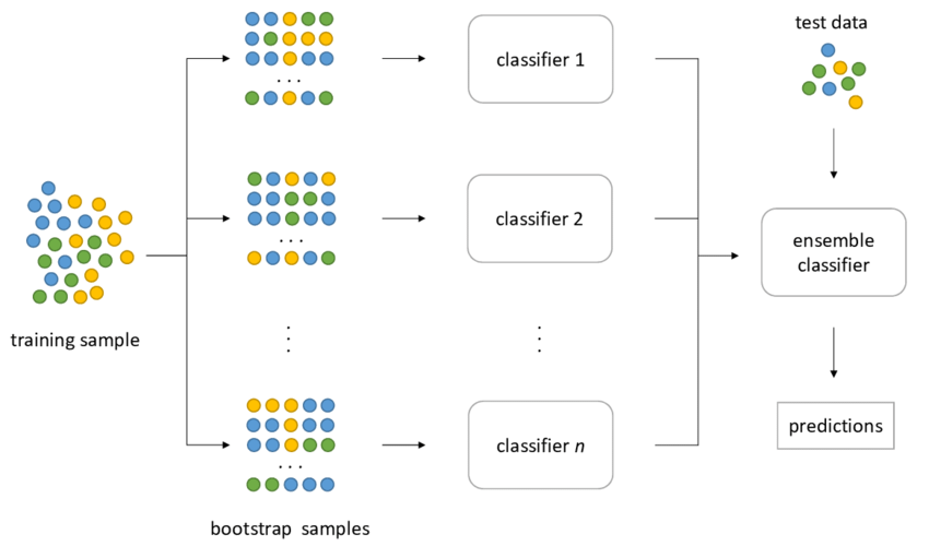
It all starts from a Decision Tree algorithm. As we all know Decision Tree is an extremely useful machine learning algorithm which solves both regression and classification style problems. It can also show the user it’s decision path which is quite useful – as well as handle a wide range of features (both numeric and categorical). The only problem is … overfitting. That is why Breiman suggested to apply the bagging technique:

Consider we have train X (features) and y (labels). Breiman suggested to randomly draw n samples from X and fit Decision Tree on this data set and repeat this procedure m times. As a result we have m different Decision Trees which were fitted on different sub-samples of X which makes trees more diverse. The final prediction would be the average prediction among m Decision Trees. Random Forest algorithm went even further by taking random feature subset to make trees even more diverse.

Bagging and Random Forest techniques have shown remarkable results on out-of-sample data sets being much less prone to be overfit. Actually we can find the same pattern in human behavior: when a person doesn’t know what to do, he usually asks for advice from different people to analyze different opinions and make the final decision.

The Bagging technique is extremely useful in finance because it directly tackles the issue of overfitting which is the main problem in quantitative finance modelling. However, why then even Random Forests fail when it comes to modelling financial processes?

Label concurrency

The core assumption of almost every classic machine learning algorithm is the so called ‘i.i.d’ of samples which is ‘Independent.Identically.Distributed’. Today we will talk about samples Independency.

Face and voice recognition, spam classification, image classification, and fraud detection are problems solved by supervised machine learning algorithms. In all of these problems samples are independent, however it is not the case of financial machine learning.

As you remember from triple-barrier labeling, sometimes label $i$ which was generated on $t$ can be triggered on $t+5$ and label $i+1$ which was generated on $t+1$ can be triggered on $t+3$ . In this example we can’t say that these two samples are independent because sample $i$ uses the information from $t+1, t+2, t+3$ which is also used by sample $i+1$ . To give you more intuition consider the example from the book ‘Advances in Financial Machine Learning’ by Marcos Lopez de Prado:

For example, you can obtain blood samples from a large number of patients, and measure their cholesterol. Of course, various underlying common factors will shift the mean and standard deviation of the cholesterol distribution, but the samples are still independent: there is one observation per subject. Suppose, you take those blood samples, and someone in your laboratory spills blood from each tube into the following none tubes to the right. That is, tube 10 contains blood from patient 10, but also blood from patients 1 through 9. Tube 10 contains blood from patient 11, but also from patients 2 through 10, and so on. Now you need to determine the features predictive of high cholesterol (diet, exercise, age, etc.) without knowing for sure the cholesterol level of each patient. That is the equivalent challenge that we face in financial ML, with the additional handicap that the spillage pattern is non-deterministic and unknown. Finance is not a plug-and-play subject as it relates to ML applications. Anyone who tells you otherwise will waste your time and money.

(source: Marcos Lopez de Prado: ‘Advances in Financial Machine Learning’ p.60)

To solve this problem we need to introduce the concept of concurrency.

We say that $y_i$ and $y_j$ are concurrent at $t$ if they are a function of at least one common return at $r_{t-1,t}$ . In our example above, labels $i$ and $i+1$ are concurrent at $t+1,t+2,t+3$ .

The level of blood sample impurity from the example would be measured by concurrency. The opposite measure of concurrency is uniqueness. We can use triple-barrier events and the closing price series data set to calculate the uniqueness of each label using get_av_uniqueness_from_tripple_barrier(triple_barrier_events, close_series, num_threads) function from mlfinlab package.

This function yields series with uniqueness of each sample, if you take average of that series you have an estimate of how ‘pure’ you dataset is. The higher the average value the purer and better your data set is, the maximum possible value is 1.

How does concurrency relate to sampling, bagging and RandomForest? Now we know that financial data sets are not independent, some labels are purer than others. It is almost impossible to make a financial machine learning data set which has independent labels, however, what we can do is to draw random samples during bagging procedure of Random Forest in such a way that we maximize the uniqueness of subsamples which are used as training sets for Decision Trees. This is called Sequential Bootstrapping !

If we refer to the blood example, we have our blood samples (read: triple-barrier events) and we do know what samples contain less information from other blood samples (using label start time and end time) which means that these samples are purer, than others. We would like to generate random samples in such a way that we still get random and diverse sub-samples, but on the other hand average purity (read: uniqueness) is maximized. Let’s understand how Sequential Bootstrapping works on toy example from the book.

Sequential Bootstrapping

Consider a set of labels ${y_i}, i = 0,1,2$ . Where:

label $y_0$ is a function of return $r_{0,2}$
label $y_1$ is a function of return $r_{2,3}$
label $y_2$ is a function of return $r_{4,5}$

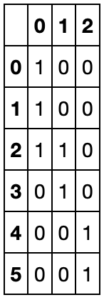
The first thing which we need to do on the first step is to build indicator matrix. The rows of the matrix correspond to the index of returns which were used to label our data set and columns correspond to samples. Initially, the indicator matrix consists of zeros so we need to fill it. We loop through samples and if $return_i$ was used to label $j$ then $matrix[i, j] = 1$ . In our case indicator matrix is:

Generating the indicator matrix is a computationally complex operation. If you take the original implementation of indicator matrix from the book, then generating an indicator matrix from 5000 triple-barrier events would take 1hour 15 minutes which is extremely long, furthermore the amount of time grows exponentially with number of samples.

We did however manage to get about a x30000 speedup! Here is the performance comparison table (2.9 GHz Intel Core i5, 4 cores):

number of samples
50
50
100
100
1000
1000
5000
5000

algorithm
original
mlfinlab
original
mlfinlab
original
mlfinlab
original
mlfinlab

time (ms)
17
3.47
49
4.72
24320
26
450253
151

The process of sequential bootstrapping is even more complex which is why our team also decided to increase its performance massively (by modifying the algorithm complexity structure, using recursive mean calculation, numba and multi-threading) so that it can be used in real-life applications where training data sets can reach millions of records. Now the performance of Sequential Bootstrapping can be increased by increasing the number of processor cores.

number of samples
10
10
50
50
100
100
1000
1000

algorithm
original
mlfinlab
original
mlfinlab
original
mlfinlab
original
mlfinlab

time (ms)
611
24
28500
50.6
180200
89.9
172800000
10900

As you can see from indicator matrix, the least overlapping label is #2.

After generating the indicator matrix, the user can simply apply seq_bootstrap function and generate sequentially bootstrapped samples! The whole process of Sequential Bootstrapping is described in Jupyter notebook in research repo: link.

If you apply seq_bootstrap function on an indicator matrix several times, you will see that label #2 is the most common in resulting subsamples.

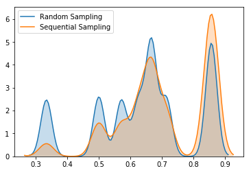
In order to ensure that Sequential Bootstrapping really increases average label uniqueness, let’s perform 10000 iterations using standard random sampling and Sequential Bootstrapping, and plot the histogram of average uniqueness using both methods.

Random sampling vs Sequential Bootstrapping

Researcher can use SequentiallyBootstrappedBaggingClassifier, SequentiallyBootstrappedBaggingRegressor which extend sklearn’s BaggingClassifier and BaggingRegressor in order to train the model using Sequential Bootstrapping sampling. The user simply needs to set samples_info_sets (which is the triple_barrier_events.t1 series), price bars as the algorithm input parameters and simply run the fit function!

Conclusion

SequentiallyBootstrappedBagging is a powerful technique which tackles the problem of label dependency by sampling the least concurrent labels. The sequential bootstrap scheme has the advantage that overlaps (even repetitions) are still possible, but decreasingly likely. In this case samples will be much closer to IID than samples drawn from the standard bootstrap method. (source: Advances in Financial Machine Learning, p.64)

Another advantage of Sequentially Bootstrapped Classifier is less inflated out-of-bag score which gives the better estimate of out-of-sample score.