Pairs Trading with Stochastic Control and OU process

by Vijay Nadimpalli

Join the Reading Group and Community: Stay up to date with the latest developments in Financial Machine Learning!

LEARN MORE ABOUT PAIRS TRADING STRATEGIES WITH “THE DEFINITIVE GUIDE TO PAIRS TRADING”

The concept of pairs trading is pretty straightforward. As described in [Gatev et al. (2006)], we first find two stocks that have moved together historically and then monitor the spread between these stocks. If the prices of the two stocks diverge, we short the winner and go long on the loser, hoping that these prices converge in the future. If the spread is mean reverting, it will revert to its historical mean. Then, the positions are reversed and a profit can be made.

There are various frameworks that could be used to identify a pair of stocks and build pairs trading strategies. In this article, we will be discussing a couple of papers related to stochastic control based approaches, which had the highest impact in this domain. We will not be discussing pairs selection techniques here, and interested readers can refer to the Stock Selection Methods using Copula and Machine Learning for Pairs Selection articles. The objective of these methods is to identify the optimal portfolio holdings in the legs of a pairs trade compared to other available assets. Stochastic control theory is used to determine value and optimal policy functions for this portfolio problem. It does sound a bit complicated, but, I’ll try to keep things simple and explain the intuition behind how and why these methods work.

What is an arbitrage strategy?

Let’s assume we have a couple of stocks that move closely together. For example, we could consider the case of the same stock trading in different exchanges. The price of this stock in both these exchanges will be similar as they are defined by the same underlying dynamics and have the same payoff. In the ideal world, the price of the stock should be the same irrespective of the exchange. But, our world is far from ideal. Due to the inherent frictions in the market, there may be significant divergence in the prices for extended periods of time. Eventually, this divergence in price should evaporate as people make moves to exploit this.

Arbitrageurs(people who exploit market inefficiencies) can earn profits by taking offsetting positions in these relatively mispriced securities. But, the mispricing could also become worse and can result in significant losses. Understanding these risks and how they might impact the positions an investor is willing to take will be crucial and is an important discussion point of this article.

Stochastic Control Strategy by Jurek et al.

Introductory financial textbooks tend to simplify the concept of arbitrage, where we can seemingly generate profits out of thin air without any initial investment. Unfortunately, exploiting real world mispricings requires thinking about some combination of both horizon and divergence risk. Horizon risk is associated with the uncertainty about the time at which the mispricing will disappear. The mispricing can also significantly increase before converging, and the risk associated with this phenomenon is called divergence risk. An OU process is used to capture these two forms of risk. Horizon risk can be measured by the uncertainty over the length of time that will elapse before the spread’s return to its long-run mean. Divergence risk, on the other hand, can be measured by the variance of the distribution of the running maximum (minimum) of the spread between its current value and its first hitting time to the long-run mean.

Next, we move on to looking at the type of investor that we are interested in. In [Jurek et al. 2007] the authors focus on two types of utility functions that can be used to model the preferences of investors. CRRA utility is defined over wealth at a finite horizon and Epstein-Zin utility is defined over intermediate cash flows(e.g fees).

What do these utility functions mean?

Utility functions assign a numerical value to the various possible outcomes which arise as a result of the various investor options. Normally the outcome will be measured in terms of resulting wealth and the utility function will be a function of wealth.

Relative risk aversion is denoted by $R(W) = \frac{-W.U''(W)}{U'(W)}$ , where $U(W)$ is the utility function of the investor. The first investor we look at has a constant relative risk aversion and maximizes the discounted utility of terminal wealth. As the name implies, for this type of utility function, $R(W) = \gamma$ , where $\gamma$ is a constant.

The corresponding value function $V_t$ for this investor is:

$V_{t}=\sup E_{t}\left[e^{-\beta(T-t)} \frac{W_{T}^{1-\gamma}}{1-\gamma}\right]$

The second investor preference structure we look at is the recursive utility of Epstein and Zin (1989, 1991), which has a nice feature of allowing intertemporal substitution(the substitution of present for future production and consumption, and vice-versa), and the coefficient of relative risk aversion to vary independently. Under this preference structure, the value function of the arbitrageur is given by:

$V_{t}=\sup E_{t}\left[\int_{t}^{T} f\left(C_{s}, J_{s}\right) d s\right]$

where $f\left(C_{s}, J_{s}\right)$ is given by:

$f\left(C_{t}, J_{t}\right)=\beta(1-\gamma) \cdot J_{t} \cdot\left[\log C_{t}-\frac{1}{1-\gamma} \log \left((1-\gamma) J_{t}\right)\right]$

Intertemporal hedging demands can play a huge role in arbitrage activities in determining when arbitrageurs trade against (or with) the mispricing.

What is the parameter $\gamma$ ? This parameter denotes the coefficient of relative risk aversion. In this model, the value of this parameter is supposed to be positive. The higher the magnitude of $\gamma$ , the more risk-averse an investor is. If the value of $\gamma < 1$ , that signifies an investor that is relatively more risk taking. $\gamma = 1$ implies a log utility investor with $U(W) = ln(W)$ .

What is the reasoning behind choosing these utility functions?

The preference structures chosen are driven by the incentives of real life arbitrageurs such as a proprietary trading desk or a fund manager with a fixed investment horizon. Modelling these types of investors using a finite-horizon CRRA utility function makes sense as such investors are only interested in the distribution of their wealth at a finite time period. However, this neglects the role of management fees, which are often collected by arbitrageurs. To capture this feature, we consider the Epstein-Zin model. Another consideration of this model is that the agent is assumed to take a flat management fee, collected as a continuous stream of payments.

Building the portfolio

Alright, let’s move on to the meaty part of this article. Let’s build an optimal portfolio.

We have two processes in our portfolio: a riskless asset and the mean-reverting spread.

Spread Construction

To construct the spread for the portfolio, firstly we calculate the total return index for each asset i in the spread. The price spread is then constructed by taking a linear combination of the total return indices. These weights are estimated by using a co-integrating regression technique such as Engle-Granger.

The hedge ratio between the two stocks in the spread is fixed using the spread construction technique mentioned above. Because the value of the spread represents the price of a long-short portfolio, buying (shorting) one unit of the spread is equivalent to buying (shorting) one unit of the overvalued security and shorting (buying) one unit of the undervalued security.

Some assumptions we make when building this model:

No margin constraints, free to short.
Exclusion of transaction costs.
Frictionless, continuous-time setting.

$\begin{aligned} d B_{t} &=r B_{t} d t \\ d S_{t} &=\kappa\left(\bar{S}-S_{t}\right) d t+\sigma d Z \end{aligned}$

To calculate the parameters of the OU process, we use the closed form estimators given in Jurek et al. [2007], which were calculated from maximum likelihood estimation on the inputted training data.

# Importing required modules
import matplotlib.pyplot as plt
import pandas as pd
import numpy as np
import yfinance as yf

from arbitragelab.stochastic_control_approach import OUModelJurek

# Importing GLD and GDX daily prices from yfinance
data1 =  yf.download("GLD GDX", start="2009-03-25", end="2019-04-25")
data2 =  yf.download("GLD GDX", start="2019-04-27", end="2020-04-27")

# Using the Adj Close prices for our dataset
data_train_dataframe = data1["Adj Close"][["GLD", "GDX"]]
data_test_dataframe = data2["Adj Close"][["GLD", "GDX"]]


# Creating an object of the Jurek class
sc = OUModelJurek()

# Calling the fit method on the train dataset
sc.fit(data_train_dataframe, delta_t = 1/252)

print(pd.DataFrame(sc.describe(), columns=['Values']))

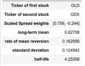
Fig. 1: Estimated parameters for the GLD-GDX pair.

Defining the wealth process

Now that we have the building blocks of our portfolio, let’s define the movements of our total wealth, represented by the wealth process.

Let $N_t$ denote the number of units of the spread that we will be holding at $t$ . Similarly, $M_t$ denotes the number of units of riskless assets held at time t.

The evolution of the wealth process which determines the budget constraints of our optimization problem is written as,

$d W_{t}=N_{t} d S_{t}+M_{t} d B_{t}-C_{t} 1\left[C_{t}>0\right] d t$

$1[C_{t}>0]$ is an indicator variable for whether intermediate consumption is taking place.

Using the above wealth process as a budget constraint for our portfolio, along with the investor-related utility functions, we can generate the optimal portfolio weight for the spread using stochastic control theory. We can derive a closed form analytical solution for this specification using stochastic dynamic programming, but the derivation is out of the scope of this article. Interested readers can refer [Jurek et al. (2007)].

The optimal portfolio weights are dynamic, which allows the investor to vary their portfolio holdings with the movements of the underlying stock prices.

For the terminal wealth problem, the optimal portfolio allocation is given by:

$N(W, S, \tau)=\left\{\begin{array}{cc} \left(\frac{\kappa(\bar{S}-S)-r S}{\sigma^{2}}\right) W & \gamma=1 \\ \left(\frac{\kappa(\bar{S}-S)-r S}{\gamma \sigma^{2}}+\frac{2 A(\tau) S+B(\tau)}{\gamma}\right) W & \gamma \neq 1 \end{array}\right.$

The functions $A(\tau)$ and $B(\tau)$ depend on the time remaining to the horizon and the parameters of the underlying model.

# In this example, we are considering the CRRA investor(utility_type = 1), with gamma = 2

# Plotting the portfolio weights of the spread asset
plt.figure(figsize=(10, 6))
scaled_weights = sc.optimal_portfolio_weights(data_test_dataframe, gamma=2, utility_type=1)
plt.plot(data_test_dataframe.index, scaled_weights, 'c-')
plt.title("Optimal allocation to the spread asset")
plt.ylabel("Weights")
plt.xlabel("Date")
plt.show()

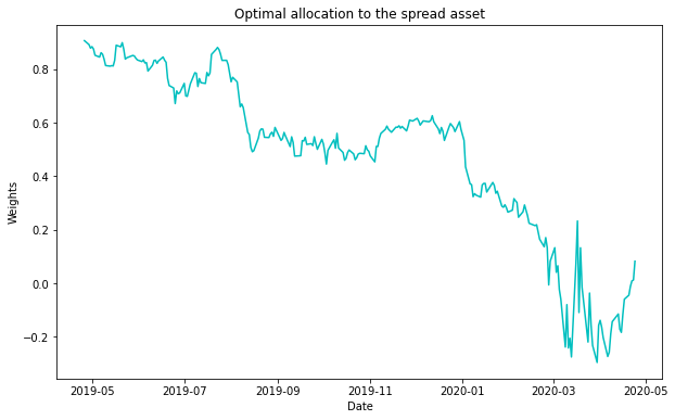
Fig. 2: Optimal Weights of the spread asset for the GLD-GDX pair considering CRRA investor.

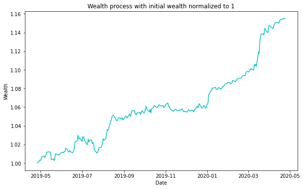
Fig. 3: Evolution of the wealth of portfolio for the GLD-GDX pair.

Effects of our trading on the underlying spread

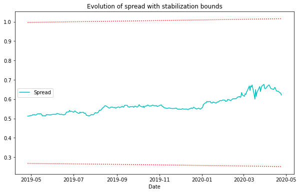
Stabilization Effect

To exploit any mispricing, as we have already mentioned, shorting one unit of the spread is equivalent to shorting one unit of the overvalued security and buying one unit of the undervalued security. Let’s suppose that there is a sudden increase in the spread between the two assets i.e. there is an increase in the difference between the prices of the underpriced and overpriced asset. If an investor increases his short position in the spread asset in response to this, he buys more of the relatively underpriced asset and goes short on the relatively overpriced asset, his trading is likely to have a stabilizing effect on the mispricing, contributing to its elimination in equilibrium.

Conversely, if the investor decreases his short position in response to the adverse shock, his trading will tend to exacerbate the mispricing. Sometimes arbitrageurs do not arbitrage. If the mispricing between the two assets is sufficiently big, a further increase in the mispricing can result in the decline of the total allocation to the spread asset in the portfolio, as the wealth effect dominates the improvement in the investment opportunities. Although a divergence in the mispricing should provide added participation by rational investors, this effect can be more than offset by the combination of the loss in wealth and the nearing of the evaluation date, which reduces the arbitrageur’s effective risk-bearing capacity. The complex tradeoff between these two effects leads to the creation of a time-varying boundary, called the stabilization region, outside of which continued divergence of the mispricing makes the rational investors cut their losses and decrease their allocations to the mispricing.

To reiterate, as long as the spread is within the stabilization region, the improvement in investment opportunities from a divergence of the spread away from its long-run mean outweighs the negative wealth effect and the arbitrageur increases his position, N, in the mean-reverting asset. When the spread is outside of the stabilization region, the wealth effect dominates, leading the agent to curb his position despite an improvement in investment opportunities.

The boundary of the stabilization region is determined by the
following inequality:

$\left| \phi(\tau) S+\frac{\kappa \bar{S}+\sigma^{2} B(\tau)}{\gamma \sigma^{2}}\right |<\sqrt{-\phi(\tau)}$

where,

$\phi(\tau) = \left(\frac{2 A(\tau)}{\gamma}-\frac{\kappa+r}{\gamma \sigma^{2}}\right)$

# In this example, we are considering the CRRA investor(utility_type = 1), with gamma = 2

S, min_bound, max_bound = sc.stabilization_region(data_test_dataframe, beta=0.1, gamma=2, utility_type=1)

# Plotting the stabilization bounds and the spread.
plt.figure(figsize=(10, 6))
plt.plot(data_test_dataframe.index, S , 'c-', label='Spread')
plt.plot(data_test_dataframe.index, min_bound, 'r:')
plt.plot(data_test_dataframe.index, max_bound, 'r:')
plt.title("Evolution of spread with stabilization bounds")
plt.xlabel("Date")
plt.legend()
plt.show()

Fig. 4: Evolution of the spread asset with corresponding stabilization bounds for the GLD-GDX pair.

Modelling in the presence of Fund Flows and Liquidity Crunches

Along with the fluctuations of asset prices, fund managers also have to deal with their client’s desire to increase or decrease their respective funds. Inconveniently, clients are most likely to withdraw funds when the performance of the fund has been poor due to a diverging spread, especially at the time when investment opportunities are the best.

To understand the effect of fund flows on the model, the authors of the paper introduced the fund flows process, $F_t$ . Let’s also assume that $\Pi_t$ , denotes the past performance of the fund. The fund flows process is modeled such that it contains a component directly proportional to the lagged performance of the fund $\Pi_t$ , and a component that is uncorrelated to past performance.

$\begin{aligned} d \Pi &=\tilde{N} d S+(W-\tilde{N} S) r d t \\ d F &=f d \Pi+\sigma_{f} W d Z_{f} \\ d W &=d \Pi+d F=(1+f) d \Pi+\sigma_{f} W d Z_{f} \end{aligned}$

Here, $\tilde{N}$ is the optimal policy that we are trying to calculate.

Let’s look at the correlation between the fund flow $f$ and realized performance $\Pi$ , which reveals some interesting details that show the intuition behind modeling the fund flows in this manner.

$\rho_{\mathrm{II}, F}=\frac{f}{\sqrt{f^{2}+\frac{\sigma_{f}^{2}}{\sigma^{2}} \cdot\left(\frac{N}{W}\right)^{-2}}}$

As can be seen from the equation above, the correlation increases with the magnitude of $\frac{{N}}{W}$ which becomes especially large outside the stabilization region. This implies that the correlation between fund flows and fund performance increases as the spread diverges from its long-run mean. Further, a fund that has experienced losses due to the divergence of the mispricing is also likely to experience loss in fund flow(outflows) from client withdrawals. And, this aspect of the model ensures that it captures the possibility of a liquidity crunch in which, after sustaining extreme losses, old investors exit the market when the investment opportunity set is most attractive.

Finally,

$\tilde{N}(S, \tau)=\left(\frac{1}{1+f}\right) \cdot N(S, \tau)$

where $N(S, \tau)$ is the optimal policy function in the problem without fund flows.

This surprisingly elegant solution leads to some interesting inferences. The component of fund flow which depends on the past performance of the fund increases the volatility of wealth by a factor of $(1+f)$ . This makes the fund manager decrease the amount of risk taken on by the underlying strategy.

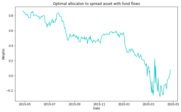
# Plotting the portfolio weights of the spread asset with fund flows
plt.figure(figsize=(10, 6))
plt.plot(data_test_dataframe.index, sc.optimal_portfolio_weights_fund_flows(data_test_dataframe, f=0.05,
                                                                            gamma=2), 'c-')
plt.title("Optimal allocation to spread asset with fund flows")
plt.ylabel("Weights")
plt.xlabel("Date")
plt.show()

Fig. 5: Optimal Weights with fund flows of the spread asset for the GLD-GDX pair considering CRRA investor.

Results

In this section, we look at the results of a pair of stocks in the group called the Siamese Twins. These are “firms that for historical reasons have two types of shares with fixed claims on the cash flows and assets of the firm.” Specifically, we look at the backtesting results from the Royal Dutch / Shell Transport pair with the dataset from the time period spanning 1990 to 2005.

To generate the results, as Jurek et al. [2007] suggest, we consider a 2500 day rolling window to estimate the parameters of the OU process and use these estimates to trade on the next 250 days.

# Loading the Shell-Royal Dutch Petroleum close prices dataset from 1990 to 2005.
data = pd.read_csv('shell-rdp-close_USD.csv', index_col='Date').ffill()
data.index = pd.to_datetime(data.index, format="%d/%m/%Y")

# Creating an object of class and calling the plotting method on the dataset.
sc = OUModelJurek()
sc.plot_results(data, num_test_windows = 5, figsize=(10, 6), fontsize=10)

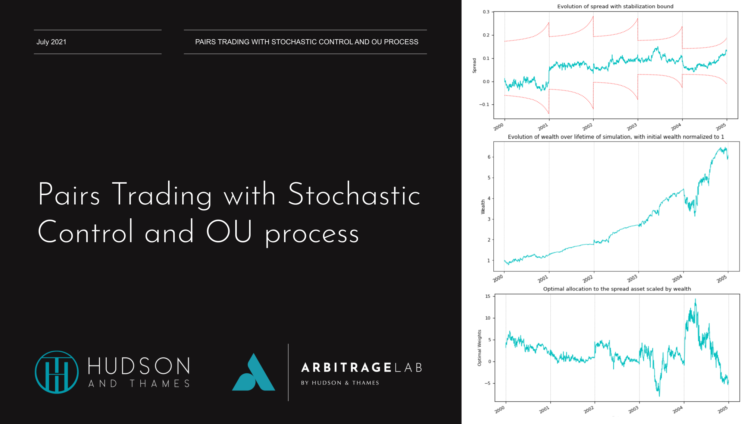
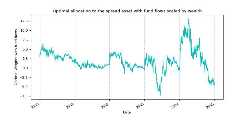
Jurek model optimal allocation weights with fund flows

Fig. 6: Optimal Weights of the spread without and with fund flows.

Looking at the optimal weights plots above, these are identical except for the values on the y-axis of the plot with fund flows, which are a fraction of the optimal weights without fund flows. This is straightforward to see from the optimal portfolio weights with the fund flows equation.

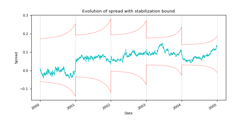
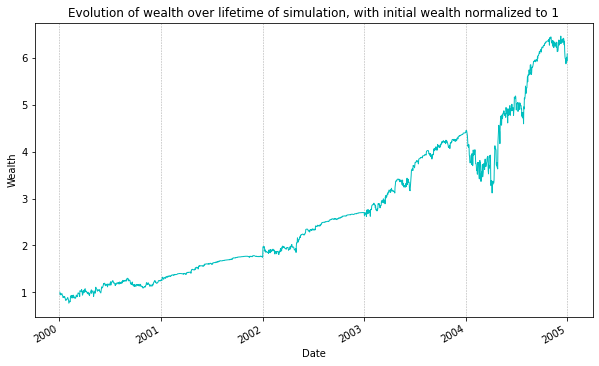
Fig. 7: Stabilization bound and Wealth of the portfolio.

The above plot represents the total wealth of our portfolio over time. Here initial wealth of the portfolio is assumed to be 1. Over the total length of the investment period, the wealth of the portfolio has increased 6-fold, which is a pretty decent profit, even though there are some drawdowns over the lifetime of the simulation.

Stochastic Control Strategy by Mudchanatongsuk et al.

Let’s take a look at a different approach to pairs trading using stochastic control approaches. Here, we model the difference in log-price of a pair of stocks as an OU process. Also, we assume that an investor’s preference can be represented by the power utility function.

Let $A(t)$ and $B(t)$ denote respectively the prices of the pair of stocks $A$ and $B$ at time $t$ . Assume that stock $B$ follows a geometric Brownian motion,

$d B(t)=\mu B(t) d t+\sigma B(t) d Z(t)$

Another difference from the previous model is that the spread is constructed as the log-difference between the two stock prices. The spread is modeled using an OU process,

$X(t) = \ln(A(t)) − \ln(B(t))$

$d X(t)=k(\theta-X(t)) d t+\eta d W(t)$

As before, we are interested in calculating the final wealth of our portfolio at the end of the investment period. Before we can calculate that, we need to look at the movements of the wealth of our portfolio through time.

The wealth dynamics are given by the following equation,

$d V(t)=V(t)\left\{h(t) \frac{d A(t)}{A(t)}+\tilde{h}(t) \frac{d B(t)}{B(t)}+\frac{d M(t)}{M(t)}\right\}$

where $V(t)$ is the value of the pairs-trading portfolio at time $t$ . Here, $h(t)$ and $\tilde{h}(t)$ denote the portfolio weights for stock $A$ and stock $B$ . One important consideration we make in this model, as was the case with the previous model, is that we restrict ourselves to a delta neutral portfolio. What this means is that we are only allowed to go short one of them and long the other in equal dollar amount. Therefore,

$h(t) = -\tilde{h}(t)$

This consideration greatly simplifies the model. Next, to represent the investor preferences, we make use of the power utility function $U(x) = \frac{1}{\gamma} x^\gamma$ , with $\gamma < 1$ . Finally, we move on to formulate the portfolio optimization problem.

Our objective is to find the portfolio weights $h(t)$ which would maximize the expected utility at the end of our investment period, i.e, at final time $T$ ,

$\begin{aligned} \sup _{h(t)} \quad & E\left[\frac{1}{\gamma}(V(T))^{\gamma}\right] \\[0.8em] \text { subject to: } \quad & V(0)=v_{0}, \quad X(0)=x_{0} \\[0.5em] d X(t)=& k(\theta-X(t)) d t+\eta d W(t) \\ d V(t)=& V(t)((h(t)(k(\theta-X(t))+\frac{1}{2} \eta^{2}\\ &+\rho \sigma \eta)+r) d t+\eta d W(t)) \end{aligned}$

To solve the above optimization problem, HJB equation along with the proper ansatz is used to obtain closed form solution. Let’s not go into too much detail regarding this derivation, as that is not the focus here. Interested readers can refer Jurek et al. [2007] for a detailed look at how we can derive the closed form solutions for optimal portfolio weights.

Finally, the optimal weights are given by,

$h^{*}(t, x)=\frac{1}{1-\gamma}\left[\beta(t)+2 x \alpha(t)-\frac{k(x-\theta)}{\eta^{2}}+ \frac{\rho \sigma}{\eta}+\frac{1}{2}\right]$

The parameters in this model are estimated using the maximum likelihood estimation.

Results

Let’s take a look at the results obtained from backtesting this strategy on the GLD-GDX pricing data from 2010 to 2020.

from arbitragelab.stochastic_control_approach import OUModelMudchanatongsuk

# Importing GLD and GDX daily prices from yfinance
data1 =  yf.download("GLD GDX", start="2010-01-01", end="2017-12-31")
data2 =  yf.download("GLD GDX", start="2018-01-01", end="2020-01-01")

# Using the Adj Close prices for our dataset
data_train_dataframe = data1["Adj Close"][["GLD", "GDX"]]
data_test_dataframe = data2["Adj Close"][["GLD", "GDX"]]

# Creating an object of the Mudchanatongsuk class
sc = OUModelMudchanatongsuk()

# Calling the fit method on the train dataset
sc.fit(data_train_dataframe)

print(pd.DataFrame(sc.describe(), columns=['Values']))

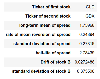
Fig. 8: Estimated parameters for the GLD-GDX pair.

Given above are the estimated parameters calculated on the GLD-GDX pair of stocks. The half-life of the spread is calculated from the rate of mean reversion.

# In this example, we consider gamma = -10

# Plotting the portfolio weights of the spread asset
plt.figure(figsize=(10, 6))
weights = sc.optimal_portfolio_weights(data_test_dataframe, gamma = -10)
plt.plot(data_test_dataframe.index, weights, 'c-')
plt.title("Optimal allocaton to the spread asset")
plt.ylabel("Weights")
plt.xlabel("Date")
plt.show()

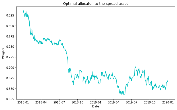
Fig. 9: Optimal Weights of the spread asset for the GLD-GDX.

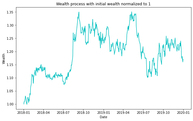
Fig. 10: Evolution of the wealth of portfolio for the GLD-GDX pair.

The figure above shows the evolution of the wealth of the portfolio with time. Initial wealth is normalized to 1, and there is a profit made in the two years.

Comments

So, in this article, we looked at two stochastic control based pairs trading approaches, with the highest impact in this domain. Implementations of both these approaches can be found in the stochastic_control_approach submodule inside arbitragelab. Feel free to experiment with these methods using various input datasets and parameters. Relevant documentation along with Jupyter notebooks are available via Hudson&Thames Client Portal.

It is important to keep in mind that, these models only represent a partial reality as they are devoid of institutional frictions. For instance, these models assume full use of short proceeds and exclude borrowing and transaction costs. The trading results presented in the article should be looked at as an upper bound on the potential gains that can be attained from exploiting arbitrage using these pairs trading techniques.

References

- Gatev, Evan, William N. Goetzmann, and K. Geert Rouwenhorst, 2006, Pairs Trading: Performance of a Relative Value Arbitrage Rule, Review of Financial Studies, 19, 797-827.
- Jurek, J.W. and Yang, H., 2007, April. Dynamic portfolio selection in arbitrage. In EFA 2006 Meetings Paper.
- Krauss, C., 2017. Statistical arbitrage pairs trading strategies: Review and outlook. Journal of Economic Surveys, 31(2), pp.513-545.
- Mudchanatongsuk, S., Primbs, J.A. and Wong, W., 2008, June. Optimal pairs trading: A stochastic control approach. In 2008 American control conference (pp. 1035-1039). IEEE.