Copula for Statistical Arbitrage: A C-Vine Copula Trading Strategy

by Hansen Pei

Join the Reading Group and Community: Stay up to date with the latest developments in Financial Machine Learning!

This is the sixth article of the copula-based statistical arbitrage series. You can read all the articles in chronological order below. In this series, we dedicate articles 1-3 to pairs-trading using bivariate copulas and 4-6 to multi-assets statistical arbitrage using vine copulas.

LEARN MORE ABOUT PAIRS TRADING STRATEGIES WITH “THE DEFINITIVE GUIDE TO PAIRS TRADING”

READ NOW

Introduction

In this article we introduce a vine copula-based strategy for statistical arbitrage from [Stübinger et al., 2018] with some analysis, then we generalize their framework and suggest what can be modified. With the power of vine copula, we can directly model the relationships among multiple stocks. We want to trade based on the information generated from a vine copula model. Similar to those traditional bivariate copulae approaches in pairs trading, we will use the conditional (cumulative) probability to gauge whether a target stock is underpriced or overpriced against other stocks, and then generate trading signals based on them from a mean-reversion bet.

We aim to cover the following topics:

Quick overview of copula-based trading strategies.
Idea and typical workflow of the C-vine copula approach.
Strategy assumptions and details.
Comments and some analysis for this strategy.

For a better understanding of vine copulas, we suggest going through Copula for Statistical Arbitrage: Stocks Selection Methods first, as we will not repeat all the details of definitions and the intuitions behind them.

Overview of Copula-Based Strategies

One key advantage the copula has is its ability to directly model the relation between two (or multiple) random variables, regardless of their marginal distributions. For example, in the pairs trading framework, each stock may resemble a log-normal distribution, but the way they are related may follow a Gaussian copula (No tail dependence. This is usually not realistic because stocks tend to co-move when the market swings in large movements.) or a Student-t copula (Symmetric upper and lower tail dependence. Also not quite realistic because stocks tend to have stronger co-moves when the market goes down). When the copula, the “link” between the two random variables changes, their joint density changes as well.

Such generality grants great flexibility for copula-based methods. Although to the best of our knowledge, the trading strategies available in the literature are exclusively on mean-reversion methods, and the C-vine copula strategy we are going to go over is also a mean-reversion bet, logically copula can model a lot more than just mean-reversion.

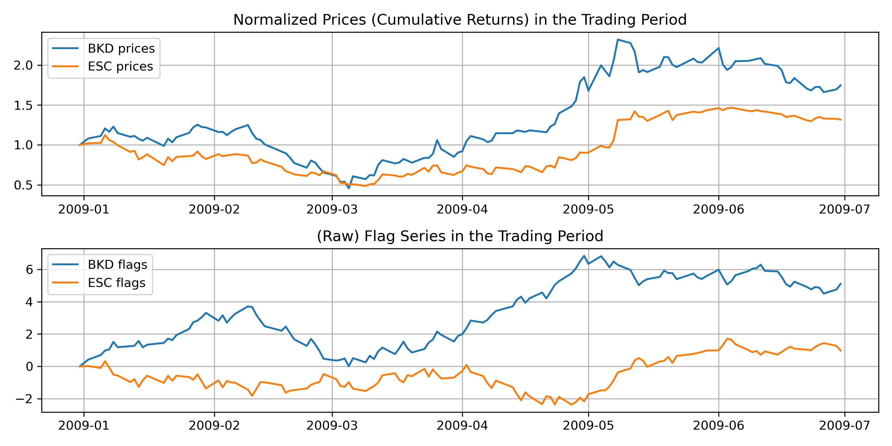
Fig 1. The plot of normalized prices (top) and CMPI series (bottom) of two stocks. Notice the similarity of shape.

Most copula-based strategies also follow the framework proposed in [Xie et al. 2014] by using returns data, in which they calculate the conditional cumulative density, also called Mispricing Index (MPI), and its cumsum (CMPI). This quantity is (hopefully) a reflection of the relative mispricing level of one stock against the rest, given their current returns data. Since it is calculated from a copula, it is, therefore, a model-dependent quantity, and it generates a CMPI time series for each stock that resembles its price time series. We can therefore think of most copula strategy as follows:

Copula translates the price time series into the relative mispricing level time series.

Compared to the price series themselves, the CMPI series takes into account historical data, and due to the nature of copula, the extreme co-moves are naturally taken into consideration (Of course you need to model their relation by a copula with tail dependence. A Gaussian copula won’t do the trick!). Therefore, with a good chance, the CMPI series include an abundance of critical information that is not present in the prices series. A good trading strategy should therefore be designed to make use of that extra bit of information.

Once we realize the above, it opens a lot of doors to adapt copula-based strategies: ALL methods that can be used for time series now can be coupled with copula. For example, with 2 assets, you can model the spread between the two CMPI series by an Ornstein-Uhlenbeck process (for whatever reason) and use an existing library to find optimal execution timing. The choices are virtually limitless. We think finding a right combination to be the key to advantage.

Why C-vine Copula?

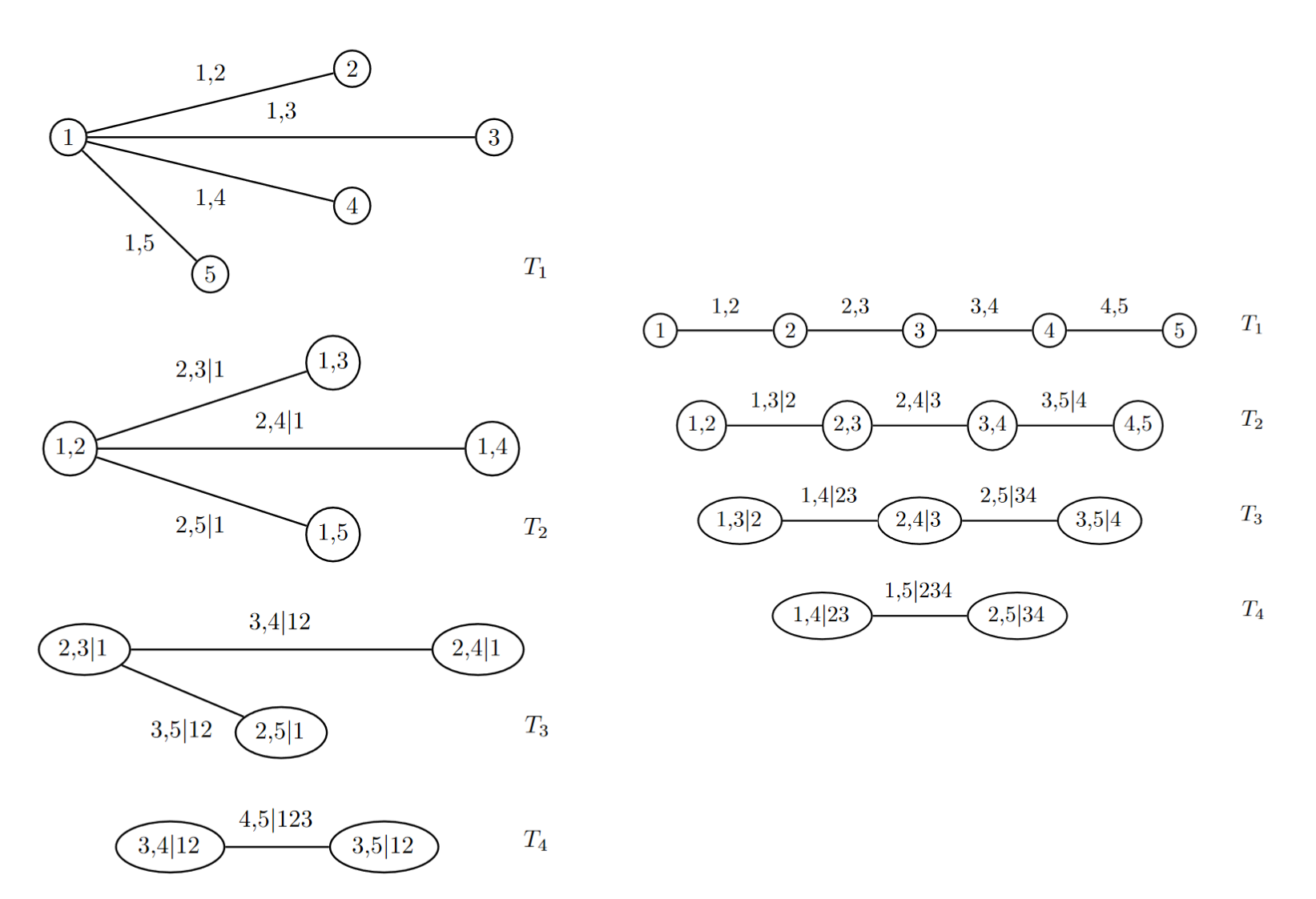
Long story short, vine copula is much more flexible than generic high-dimensional copulas. C-vine (Canonical-vine) is characterized by having a star-like graph at each level of the vine tree, representing the belief of dependence around that variable from other variables.

Fig 2: C-vine and D-vine tree. Picture from Brechmann, E. and Schepsmeier, U., 2013. Cdvine: Modeling dependence with c-and d-vine copulas in r. Journal of statistical software, 52(3), pp.1-27.

C-vine is used for the following reasons:

Model interpretability: C-vine reflects the belief of ordering variables by importance measured by the strength of dependency. A generic R-vine is difficult to interpret.
Avoiding overfitting: An R-vine may get unnecessarily complicated, and therefore overfit to current data, given that one just fits the R-vine structure by max-likelihood.
The one-vs-others trading framework we adopt: We will trade using a target stock against the rest in a stocks cohort (specifically 1-vs-3 in the ArbitrageLab implementation). It makes logical sense to let the target stock become the center in the C-vine structure.

For a more thorough comparison between C-vine, D-vine, and R-vine and a qualitative discussion of their properties, you can read the previous article Copula for Statistical Arbitrage: A Practical Introduction to Vine Copula or refer to the seminal book Analyzing Dependent Data with Vine Copulas by Claudia Czado.

Strategy Workflow

We implemented the trading strategy proposed by [Stübinger et al., 2018], along with the stock selection methods. We will focus on the strategy itself, and the details in the stock selection are included in Copula for Statistical Arbitrage: Stocks Selection Methods to keep this post within a manageable length. For now, assume we have already selected 4 stocks to form a cohort, and they are picked in a way based on their “strong interdependence” to (hopefully) benefit a mean-reverting strategy.

Step 1: Get data

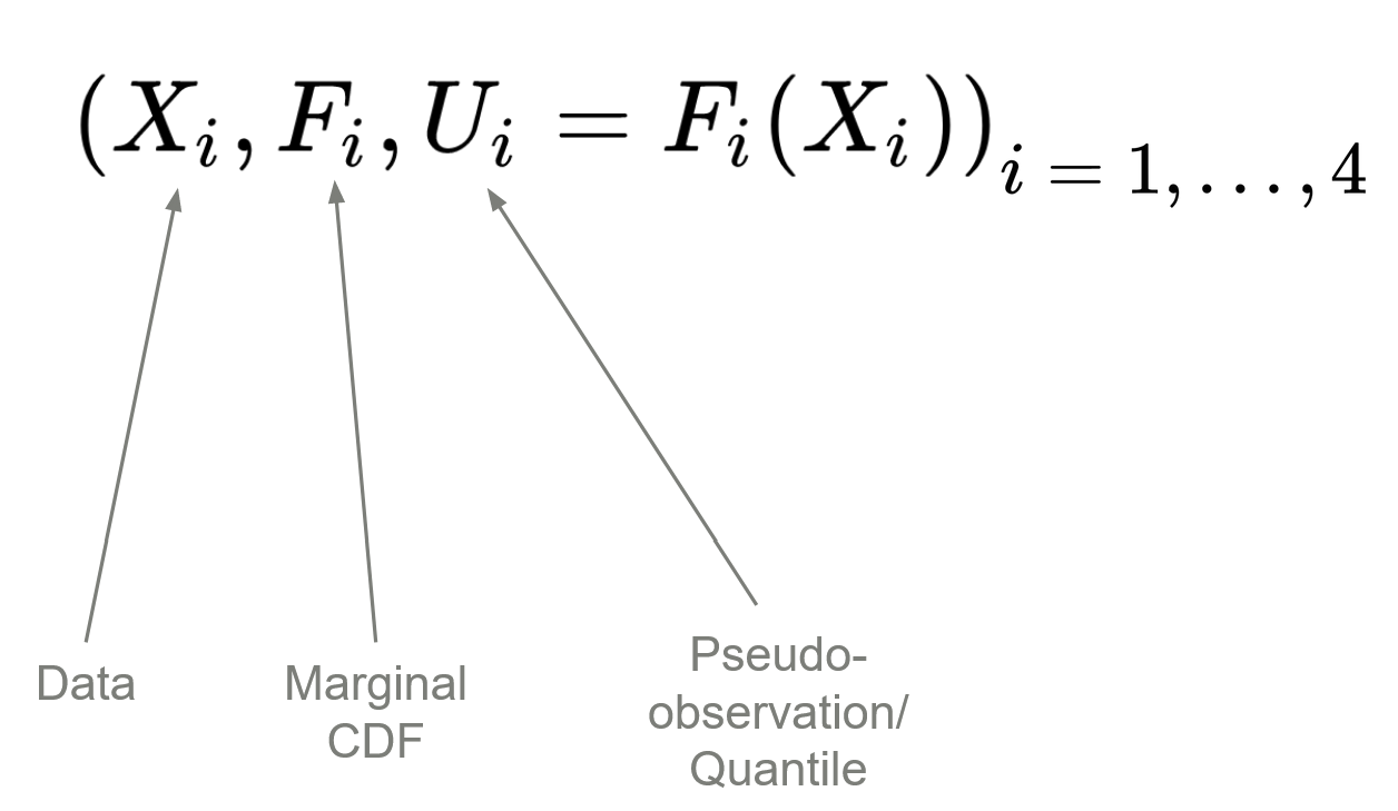
We work with stocks’ returns exclusively. We then need to translate the stocks’ returns data into their quantiles (pseudo-observations) using empirical CDFs (ECDFs). We denote the pseudo-observations as $u_i$ ‘s, and they are all uniform in $[0, 1]$ .

Fig 3. Generate pseudo-observations or quantiles and marginal ECDFs from returns data.

Step 2: Determine the C-vine Structure

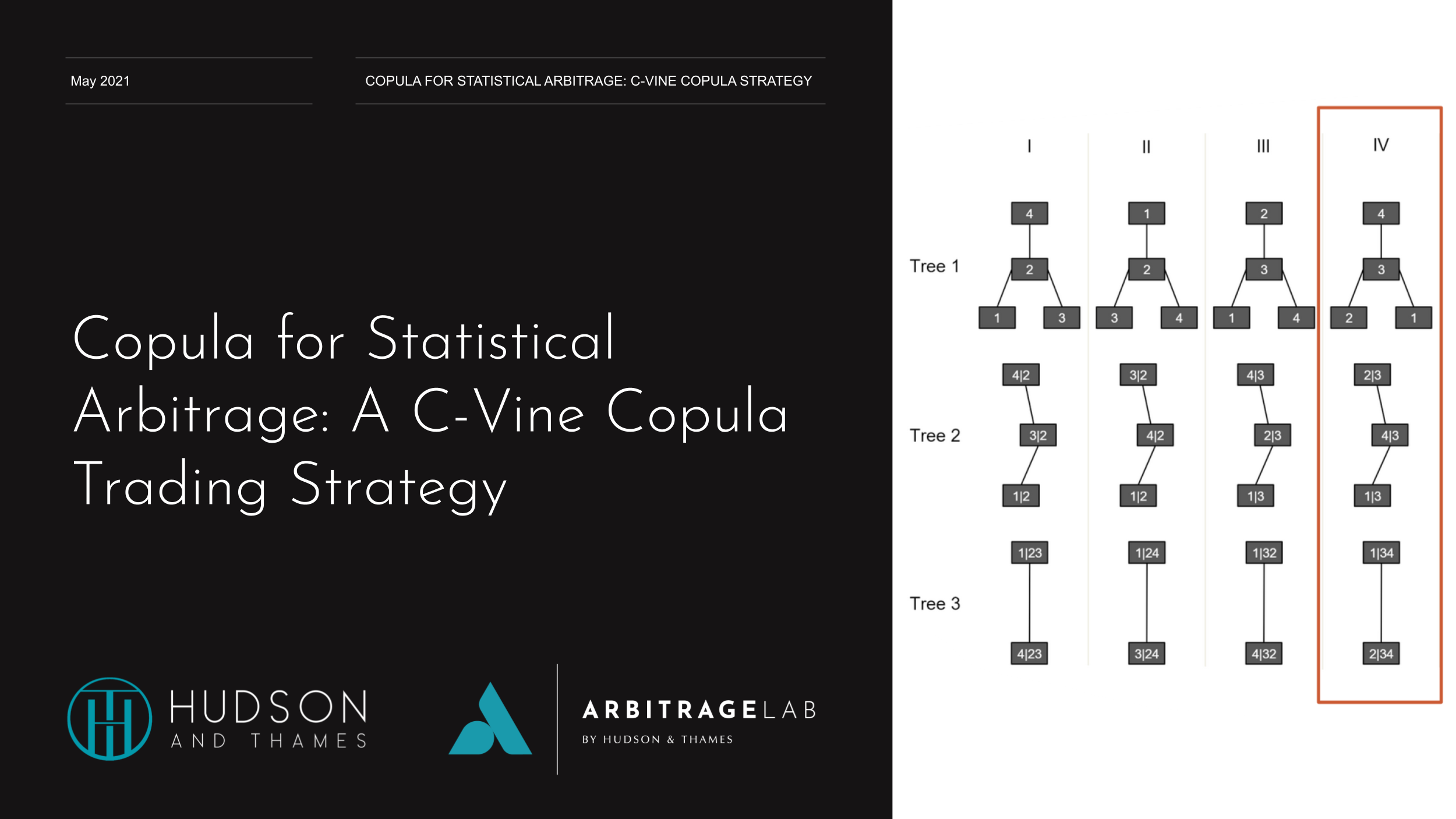
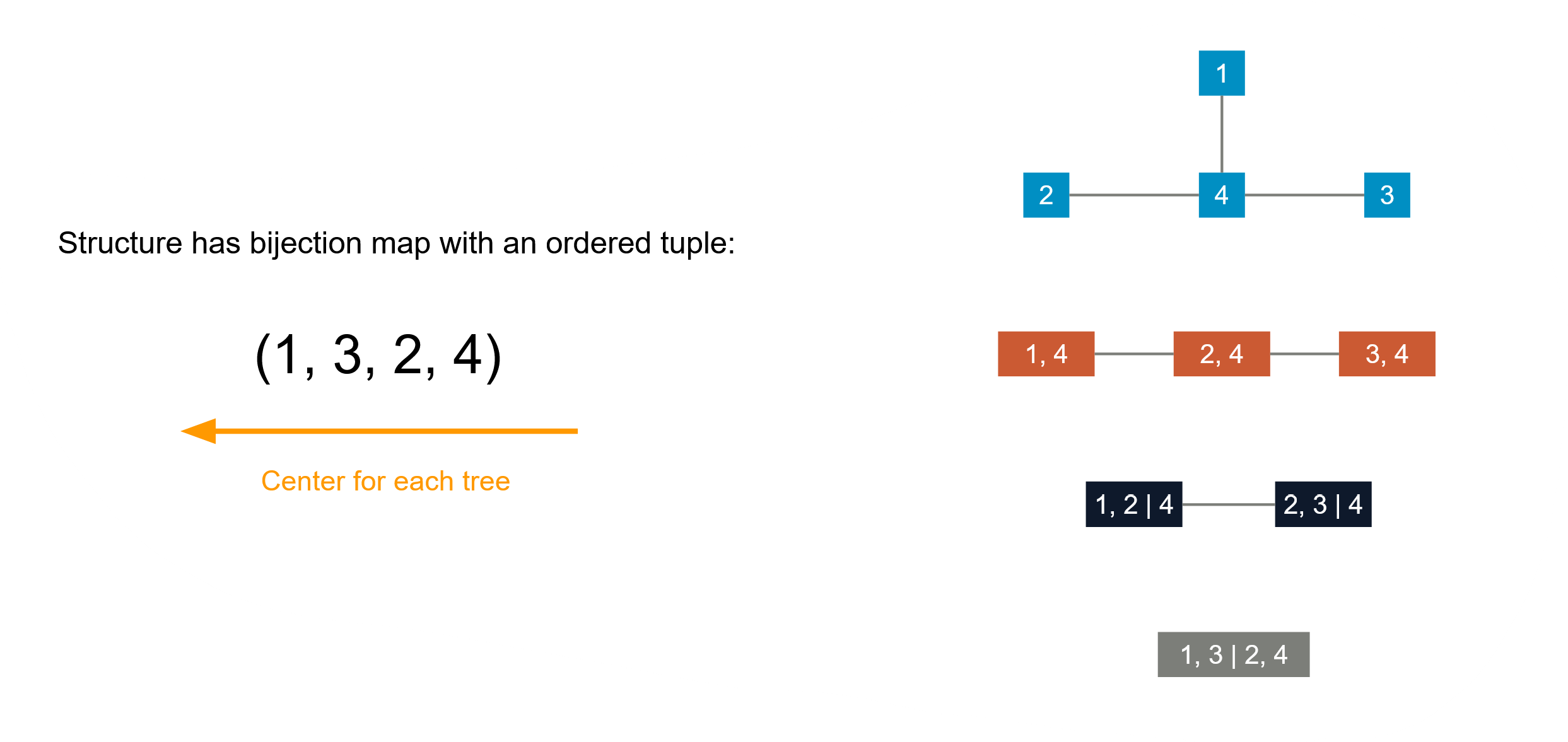
We essentially need to determine two things: what C-vine structure to use, and with a given C-vine structure what are the nodes (bivariate copulas)? Since each C-vine structure can be bijectively mapped to an ordered tuple, with each number indicating the center at each level of the tree. For example:

Fig 4. C-vine and its ordered tuple representation. In some literature, for example in [Czado et al. (2012)] it is written reversely as (4, 2, 3, 1)

To start with, there are $4! = 24$ many possible C-vine structures. Without loss of generality assuming stock 1 is our target stock. In the end, we aim to come up with this conditional density that indicates relative mispricing for stock 1 against the 3 other stocks in this cohort:

$h(u_1 | u_2, u_3, u_4) = \mathbb{P}(U_1 \le u_1 | U_2=u_2, U_3=u_3, U_4=u_4)$

If $h(u_1 | u_2, u_3, u_4) < 0.5$ then that day’s return for stock 1 is considered lower than the mean of what the history tells and vice versa, similar to the approaches in [Xie et al. 2014].

In [Stübinger et al. 2018], the authors claimed that to calculate $h(u_1 | u_2, u_3, u_4)$ , stock 1 must never be at the center of every level of the tree. Remember that a C-vine structure $(c_4, c_3, c_2, c_1)$ indicates that $c_1$ is the center for the level-1 tree, $c_2$ for level-2 and so on. Therefore, to make stock 1 never at the center (except at the tree root), it is equivalent to check each possibility generated by $(1, c_3, c_2, c_1)$ , where $(c_3, c_2, c_1)$ is a permutation of $\{2, 3, 4\}$ . Obviously, there are $3! = 6$ many ways available.

However, we think when we treat stock 1 as the key stock, it is reasonable to put stock 1 at the center of the 0-th level of the tree (thus every level), because it makes intuitive sense to model all other stocks’ and their bivariate copula densities relation given the key stock 1’s information. Stock 1 is the object of interest, and therefore should be the governing quantity here. C-vine structure intrinsically orders the marginal variables by their importance of interdependencies from its ordered tuple representation, and the target stock should be the most important (therefore at the end of the tuple). It is a bit logically inconsistent to argue that the least important stock in terms of interdependencies should become the target stock. I.e., 1 should be put at the end of the tuple, not at the beginning, and there are still 6 many possible structures for 4 stocks. Currently we provide both the implementation in [Stübinger et al. 2018] and the alternative method that puts the target stock at the center in ArbitrageLab.

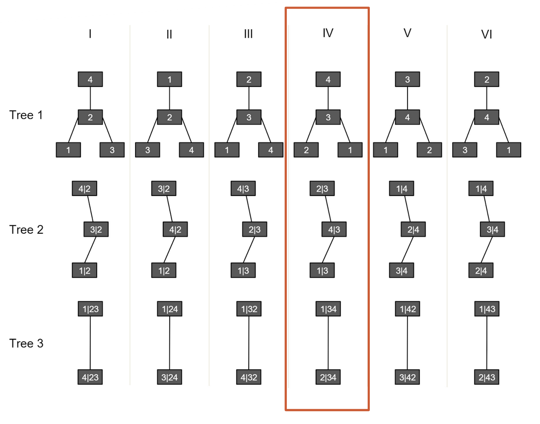
After choosing the 6 possible vine structures, we then fit every one of them and calculate the associated AIC value. We choose the final C-vine structure among candidates with the lowest AIC value. It is equivalent in this case to directly compare the log-likelihood and choose the one that constitutes the largest log-likelihood value. The exact fitting includes figuring out what type of (parametric) bivariate copula to use for every node and the parameter(s) value that fits best the data.

Fig 5. Determine the C-vine structure by AIC or maximum likelihood. Picture from [Stübinger et al. 2018]. The selected C-vine has the tuple representation (1, 2, 4, 3).

Step 3: Calculate Probability Density

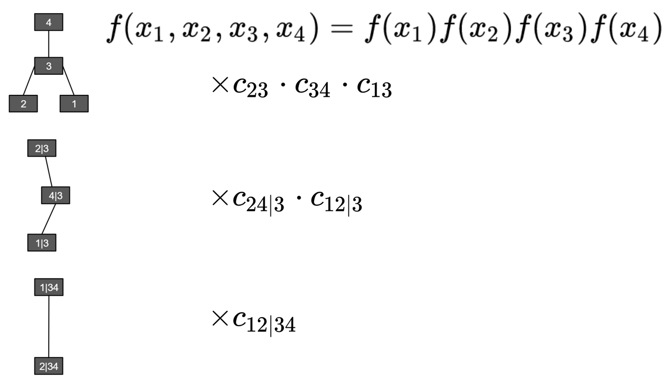
We aim to calculate $f(u_1, u_2, u_3, u_4)$ . This is straightforward once we fit the C-vine to training data. Now we are working on the trading period data. At first, we should map them into quantiles using the ECDFs trained in the training period. Then we can calculate directly the probability density for pseudo-observations, say $(u_1, u_2, u_3, u_4)$ , by calculating every node at every level of the tree. Note that each node constitutes a probability density, either marginal density (top of the tree) or the copula density (not top of the tree). And the final probability density is their product.

Fig 6: Determine the joint density $f(u_1, u_2, u_3, u_4)$ from the vine copula. Here the notation $f(x_1, x_2, x_3, x_4)$ is okay since we start from the beginning only using quantiles data, so $u_i = x_i$ .

Step 4: Calculate CMPI

We aim to calculate $h(u_1| u_2, u_3, u_4)$ , given that stock 1 is the target stock. Similarly, we can compute for other stocks if they are the target. Here we use numerical integration for this value:

(1) $\begin{align*} h(u_1 | u_2, u_3, u_4) &= \mathbb{P}(U_1 \le u_1 | U_2=u_2, U_3=u_3, U_4=u_4) \\ &= \left( \int_0^{u_1} f(u, u_2, u_3, u_4) du \right) / \left( \int_0^{1} f(u, u_2, u_3, u_4) du \right) \end{align*}$

Keep in mind that this value is model-dependent: it depends on which vine structure we are using, and the types of bivariate copulas and their parameters in each node. Some people denote the conditional probability as $h_C$ to indicate that it depends on a copula. Here we computed $h$ from the “bottom-up” by marginal integration.

One may suggest computing from “top-down” by taking partial differentiation from the copula definition $C(u_1, u_2, u_3, u_4)$ (cumulative density) similar to what we have done previously in bivariate copula models:

$h(u_1 | u_2, u_3, u_4) := \frac{\partial^3 C(u_1, u_2, u_3, u_4)}{\partial u_1 \partial u_2 \partial u_3}$

We did not choose such an approach for the following reason: Mathematically speaking it is the same. However vine copula only allows one to compute the joint density $f$ , and unlike “traditional” copula models where $C$ is defined by definition. Vine copula is constructed from point densities, not cumulative densities, and $C$ is found by integrations from $f$ . Due to the analytical complexity, the integration is usually done through Monte-Carlo. Also even if $C$ can be found analytically, taking 3 numerical partial differentiation will likely yield more issues compared to numerically integrating just along 1 marginal variable.

Step 5: Generate Signals and Trade

As we have discussed in the beginning, any method that works with financial time series can be used together with the vine copula method, since the C-vine copula generates a CMPI for each stock in the cohort. In [Stübinger et al., 2018] the author suggested a simple Z-score-based Bollinger band strategy and that is what we are introducing here to finish the post. Intrinsically once you calculated the CMPI series you can use whatever method you see fit.

For conditional probability $h=h(u_1| u_2, u_3, u_4)$ :

If $h > 0.5$ , stock 1’s return that day is higher than the historical average compared to the other 3 stocks in the cohort.
If $h < 0.5$ , stock 1’s return that day is higher than the historical average compared to the other 3 stocks in the cohort.

Therefore, we adopt the cumulative mispricing index framework. For each cohort we calculate the de-meaned cumulative sum of $h$ as $CMPI$ , and formulate the trading signal using a Bollinger band: Denote the running average of $CMPI$ in the fixed-length, moving time window as $\hat{\mu}(t)$ , the running standard deviation in the time window as $\hat{\sigma}(t)$ , and some positive constant $k$ to control the Bollinger band’s width.

Short signal: When $CMPI > \hat{\mu}(t) + k \hat{\sigma}(t)$ .
Long signal: When $CMPI < \hat{\mu}(t) - k \hat{\sigma}(t)$ .
Exit signal: When $CMPI$ crosses with $\hat{\mu}(t)$ .
Do nothing: Else.

Now we total net positions for each key stock in each cohort. Then we formulate our dollar-neutral strategy by trading
against a cheap broad-based market index such as SPY, similar to the method used in [Avellaneda and Lee, 2010].

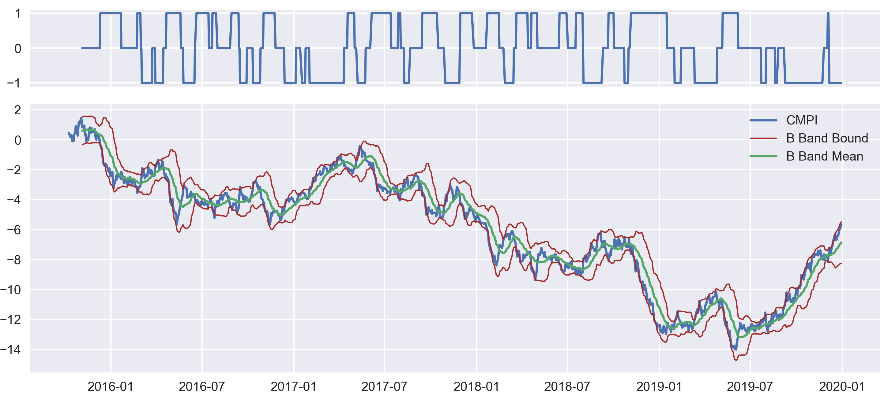
Fig 7. Positions (top) and the CMPI Bollinger band.

Comments

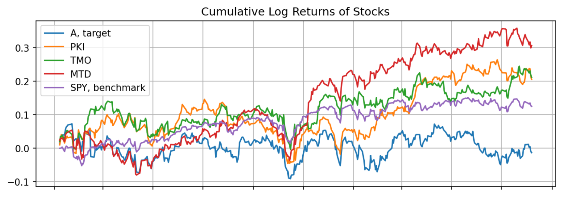
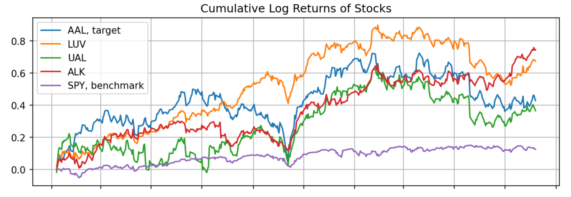
There is one caveat with the above method. A key effect to take into consideration is the way the dollar-neutral strategy is carried: instead of long/short the stocks, it trades each target stock against an index (potentially to lower cost). Therefore, everything else being equal, if a stocks cohort does not have most of its members behaving like the index, such a method will not lead to great results. Indeed, here are examples of a “good” cohort and a “bad” cohort.

Fig 8. Example of a “good” cohort: SPY behaves similarly to the cohort’s constituents.

Fig 9. Example of a “bad” cohort: SPY behaves very differently to the cohort’s constituents.

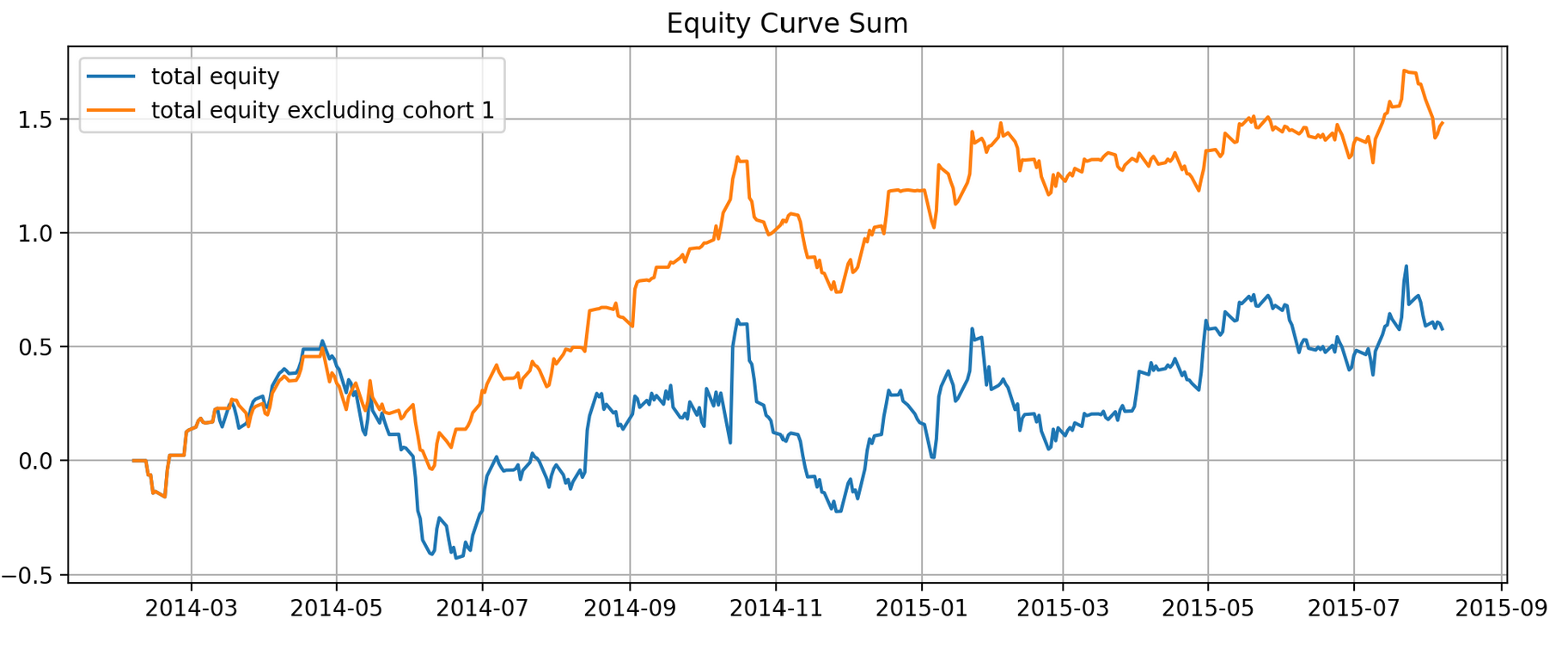
Fig 10. Equity curve with the implemented strategy. Cohort 1 in this example is the only “bad” cohort out of 4 cohorts in total.

This can happen because when selecting stocks we did not compare them with SPY. One possible way to address this is to add an extra filter simply by applying Kendall’s $\tau$ between SPY and every stock in every cohort and get rid of the cohorts with low total scores. Of course, there are other ways to be explored.

In the end, vine copula provides a very flexible approach in modeling multi-variate dependencies. It translates the original prices series to time series that reflects relative mispricing. The C-vine structure specifically highlights a dominant component at every level of the tree, ideal for the “1-vs-the rest” trading strategy for capturing statistical arbitrage among multiple stocks, which non-quant strategies often omit or are still primitive. Moreover, it can be (and should be) coupled with other methods that handle time series.

As promising as it looks, just like any other methods it inevitably bears some drawbacks:

High start-up cost: to understand this method, the user needs to understand copula modeling from scratch, and also how to interpret vine copula models from end to end.
High computation cost: For a cohort of 4 stocks and 3 years of daily training data + 1 year of test data, it takes about 30 seconds to fit and generate positions. This can hardly be optimized further since the fitting algorithm is already written in an optimized library with a compiled language, and the computation time should scale up in $O(N!)$ where N is the number of stocks in each cohort. This is just for fitting and generating positions without factoring into the time for stock selection.

In the end, we hope that we have in this series sufficiently demystified the copula concept and its applications in trading. It is still a dynamic field with lots of research potential, and we are witnessing new methods are actively being developed.

References

- Luepsen, H., 2018. Comparison of nonparametric analysis of variance methods: A vote for van der Waerden. Communications in Statistics-Simulation and Computation, 47(9), pp.2547-2576.
- Rad, H., Low, R.K.Y. and Faff, R., 2016. The profitability of pairs trading strategies: distance, cointegration and copula methods. Quantitative Finance, 16(10), pp.1541-1558.
- Stübinger, J., Mangold, B. and Krauss, C., 2018. Statistical arbitrage with vine copulas. Quantitative Finance, 18(11), pp.1831-1849.
- Mangold, B., 2015. A multivariate linear rank test of independence based on a multiparametric copula with cubic sections. FAU Discussion Papers in Economics (10).
- Schmid, F. and Schmidt, R., 2007. Multivariate extensions of Spearman’s rho and related statistics. Statistics & probability letters, 77(4), pp.407-416.
- Schmid, F. and Schmidt, R., 2007. Multivariate conditional versions of Spearman’s rho and related measures of tail dependence. Journal of Multivariate Analysis, 98(6), pp.1123-1140.
- Nelsen, R.B., 2007. An introduction to copulas. Springer Science & Business Media.
- Xie, W., Liew, R.Q., Wu, Y. and Zou, X., 2016. Pairs trading with copulas. The Journal of Trading, 11(3), pp.41-52.