Join the Reading Group and Community: Stay up to date with the latest developments in Financial Machine Learning!
Portfolio Optimisation has always been a hot topic of research in financial modelling and rightly so – a lot of people and companies want to create and manage an optimal portfolio which gives them good returns. There is an abundance of mathematical literature dealing with this topic such as the classical Markowitz mean variance optimisation, Black-Litterman models and many more. Specifically, Harry Markowitz developed a special algorithm called the Critical Line Algorithm (CLA) for this purpose which proved to be one of the many algorithms which could be used in practical settings. However, the algorithm comes with its own set of caveats –
- The CLA algorithm involves the inversion of a positive-definite covariance matrix and this makes it unstable to the volatility of the stock-market – the inverse of the covariance matrix can change significantly for small changes in market correlations.
- A second drawback of CLA ( and in-fact many methods in the previous literature) is that it is dependent on the estimation of stock-returns. In practical scenario, stock returns are very hard to estimate with sufficient accuracy and this makes it hard to quantify the results of this algorithm.
- CLA considers the correlations between the returns of all the assets in a portfolio and this leads to a very large correlation dependency connected graph where each asset is connected to all the other assets. Hence, when the algorithm calculates the inverse of the correlations, it is a computationally expensive task as all the edges of a connected graph are considered.
- Finally, not all the assets in a portfolio are correlated with each other and considering all possible correlations between all the assets in the portfolio is impractical. Assets can be grouped into categories depending on their liquidity, size, industry and region and it is only these stocks within each group that compete with each other for allocations within a portfolio. However, such a sense of hierarchy is lost in a correlation matrix where all assets are potential replacements for one another. This is a very important point since this is how many asset managers manage a portfolio – by comparing stocks sharing some similarities with each other and rebalancing them within individual groups.
All these disadvantages make CLA and other similar allocation algorithms unsuitable for practical applications and this is where Hierarchical Risk Parity (HRP) comes into the picture as it tries to address the above mentioned points and improve upon them. In the following sections, we will understand its algorithm in detail and finally end with a performance comparison with CLA.
How Hierarchical Risk Parity Actually Works?
The algorithm can be broken down into 3 major steps:
- Hierarchical Tree Clustering
- Matrix Seriation
- Recursive Bisection
Lets understand each step in detail. Note that I will use real stock data in the form of a .csv file containing stock-returns indexed by date. For a more detailed approach along with the code and the data file, please refer to this online research notebook and this Github repository for other cool notebooks.
Hierarchical Tree Clustering
This step breaks down the assets in our portfolio into different hierarchical clusters using the famous Hierarchical Tree Clustering algorithm. Specifically, we calculate the tree clusters based on the  matrix of stock returns where
  represents the timeseries of the data and
  represents the number of stocks in our portfolio. Note that this method combines the items into a cluster rather than breaking down a cluster into individual items i.e. it does an agglomerative clustering. Lets understand how the clusters are formed in a step-by-step manner:
- Given a matrix of stock returns, calculate the correlation of each stock’s returns with the other stocks which gives us an
 matrix of these correlations, ⍴
 - The correlation matrix is converted to a correlation-distance matrix
 , where,
\begin{aligned}
D(i, j) = \sqrt{0.5 * (1 – ⍴(i, j))}
\end{aligned} - Now, we calculate another distance matrix
 where, \begin{aligned}
\overline{D}(i, j) = \sqrt{\sum_{k=1}^{N}(D(k, i) – D(k, j))^{2}}
\end{aligned}It is formed by taking the Euclidean distance between all the columns in a pair-wise manner. - A quick explanation regarding the difference between and – for two assets
 and
and  ,
,  is the distance between the two assets while
  indicates the closeness in similarity of these assets with the rest of the portfolio. This becomes obvious when we look at the formula for calculating – we sum over the squared difference of distances of and from the other stocks. Hence, a lower value means that assets and are similarly correlated with the other stocks in our portfolio.
 - We start forming clusters of assets using these distances in a recursive manner. Let us denote the set of clusters as
 . The first cluster
  is calculated as, \begin{aligned}
U[1] = argmin_{(i,j)} \overline{D}(i, j)
\end{aligned}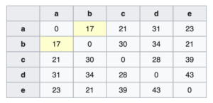 In the above figure, stocks
  and
and  have the minimum distance value and so we combine these two into a cluster.
 - We now update the distance matrix by calculating the distances of other items from the newly formed cluster. This step is called linkage clustering and there are different ways of doing this. Hierarchical Risk Parity uses single linkage clustering which means the distances between two clusters is defined by a single element pair – those two elements which are closest to each other.
- We remove the columns and rows corresponding to the new cluster – in this case we remove rows and columns for stocks and . For calculating the distance of an asset outside this cluster, we use the following formula \begin{aligned} \overline{D}(i, U[1]) = min( \overline{D}(i, a), \overline{D}(i, b) ) \end{aligned}
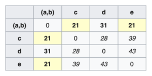 Using the above formula we calculate distances for
  ,
,  and
and  from cluster
  . \begin{aligned} \overline{D}(c, U[1]) = min( \overline{D}(c, a), \overline{D}(c, b) ) = min(21, 30) = 21\end{aligned}\begin{aligned} \overline{D}(d, U[1]) = min( \overline{D}(d, a), \overline{D}(d, b) ) = min(31, 34) = 31\end{aligned}\begin{aligned} \overline{D}(e, U[1]) = min( \overline{D}(e, a), \overline{D}(e, b) ) = min(23, 21) = 21\end{aligned}
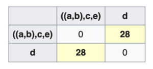
- In this way, we go on recursively combining assets into clusters and updating the distance matrix until we are left with one giant cluster of stocks as shown in the following image where we finally combine with
 .
.
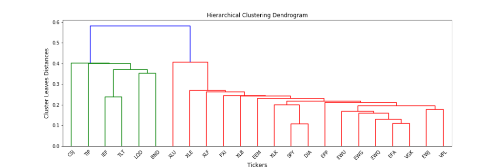
- Finally, in hierarchical clustering, the clusters are always visualised in the form of a nice cluster diagram called dendrogram. Below is the image of the hierarchical clusters for our stock data,
Matrix Seriation
In the original paper of this algorithm, this step is identified as Quasi-Diagonalisation but it is nothing more than a simple seriation algorithm. Matrix seriation is a very old statistical technique which is used to rearrange the data to show the inherent clusters clearly. Using the order of hierarchical clusters from the previous step, we rearrange the rows and columns of the covariance matrix of stocks so that similar investments are placed together and dissimilar investments are placed far apart. This rearranges the original covariance matrix of stocks so that larger covariances are placed along the diagonal and smaller ones around this diagonal and since the off-diagonal elements are not completely zero, this is called a quasi-diagonal covariance matrix

Unclustered Correlations

Clustered Correlations
The above image shows the seriated correlation matrix for our data. We see that before seriation, the asset clusters are broken down into small sub-sections and it is only after quasi-diagonalising/seriating the matrix, does the clustering structure become more evident.
Recursive Bisection
This is the final and the most important step of this algorithm where the actual weights are assigned to the assets in our portfolio.
- We initialise the weights of the assets, \begin{aligned}
W_{i} = 1, \forall i=1,…,N
\end{aligned} - At the end of the tree-clustering step, we were left with one giant cluster with subsequent clusters nested within each other. We now break each cluster into two sub-clusters by starting with the topmost cluster and traversing in a top-down manner. This is where Hierarchical Risk Parity makes use of Step-2 to quasi-diagonalise the covariance matrix and uses this new matrix for recursing into the clusters.
- Hierarchical tree clustering forms a binary tree where each cluster has a left and right child cluster
 and
and  . For each of these sub-clusters, we calculate its variance, \begin{aligned}
V_{adj} = w^{T}Vw
\end{aligned} where, \begin{aligned}
w = \frac{ diag[V]^{-1} }{ trace(diag[V]^{-1}) }
\end{aligned}This step exploits the property that for a diagonal covariance matrix, the inverse-variance allocations are the most optimal. Since, we are dealing with a quasi-diagonal matrix, it makes sense to use the inverse-allocation weights to calculate the variance for this subcluster. - A weighting factor is calculated based on the new covariance matrix \begin{aligned}
\alpha_{1} = 1 – \frac{ V_1 }{ V_1 + V_2 }; \alpha_{2} = 1 – \alpha_{1}
\end{aligned} You might be wondering how do we arrive at the above formula for the weighting factor. It comes from the classical portfolio optimisation theory where we have the following optimisation objective, \begin{aligned}
min \frac{1}{2}w^{T}\sigma w
\end{aligned} \begin{aligned}
s.t. e^{T}w = 1; e = 1^{T}
\end{aligned} where are the portfolio weights and
  is the covariance of the portfolio. For a minimum variance portfolio, the solution to the above equation comes out to be, \begin{aligned}
w = \frac{\sigma^{-1}e }{ e^{T}\sigma^{-1}e }
\end{aligned} And if is diagonal, \begin{aligned}
w = \frac{ \sigma^{-1}_{n, n} }{ \sum_{i=1}{N}\sigma^{-1}_{i, i}}
\end{aligned} Since, we only have N = 2 (2 subclusters) this equation becomes, \begin{aligned}
w = \frac{ 1/\sigma_{1} }{ 1/\sigma_{1} + 1/\sigma{2} } = 1 – \frac{ \sigma_1 }{ \sigma_1 + \sigma_2 }
\end{aligned} which is the same formula used by Hierarchical Risk Parity. - The weights of stocks in the left and right subclusters are then updated respectively, \begin{aligned}
W_1 = \alpha_1 * W_1
\end{aligned}\begin{aligned}
W_2 = \alpha_2 * W_2
\end{aligned} - We recursively execute steps 2-5 on and until all the weights are assigned to the stocks.
Notice how the weights are assigned in a top-down manner based on the variance within a sub-cluster. The main advantage of such a hierarchical weight assignment is that only assets within the same group compete for allocation with each other rather than competing with all the assets in the portfolio.
Performance of Hierarchical Risk Parity
Having understood the working of the Hierarchical Risk Parity algorithm in detail, we now compare its performance with other allocation algorithms. In particular, I will compare it with 2 algorithms – the Inverse-Variance Allocation (IVP) and Critical Line Algorithm (CLA). I will be using PortfolioLab which already has these algorithms implemented in its portfolio optimisation module. In the original paper, the author uses monte-carlo simulations to compare the performances of these algorithms, however, I will use a different method to do so.
First, let’s look at the weight allocations of the 3 algorithms for our normal portfolio,


We can see a major difference in how these 3 algorithms allocate their weights to the portfolio,
- CLA concentrates literally 99% of the holdings on the top-3 investments and assigns zero weight to all other assets. The reason behind CLA’s extreme concentration is its goal of minimising the variance of the portfolio. This makes it take a very conservative approach in allocating weights and it places emphasis on only a few of the assets.
- Inverse variance (IVP) has assigned non-zero weights to all the assets and except the top 5 holdings, its weight allocations are distributed almost uniformly. Hence, it tends to take a safer approach and tries to allocate weights almost equally to the assets.
- HRP, on the other hand, tries to find a middle ground between CLA and IVP allocations. It places more emphasis on the top 5 holdings/assets just like IVP but assigns lesser but non-uniform weights to the rest of the stocks.
- Another important fact is that both the CLA and HRP weights have very little difference in their standard deviations,
 and
and  . However, CLA has discarded half of the investment universe in favor of a minor risk reduction while HRP did not. Since, CLA has placed its emphasis on only a few of the assets, it is prone to much more negative impact by random shocks than HRP – something which we will see below.
Now, using the same stocks, I will rescale the covariance matrix of these stocks by adding some random noise from a normal distribution.


In the above image, we see that the covariances do not change drastically and the relative covariances are still the same, however there is a visible change in the values. Such a rescaling of covariances mimics the volatile nature of the stock-market and we get to see how the allocations of these algorithms are affected with such a sudden and small change in the relationships between the stocks in our portfolio.


We observe that rescaling of the variances has led to a rebalancing of the portfolios for all the three strategies. Let’s analyse the differences in this rebalancing,
- HRP tries to rebalance the reduction in allocation of one affected investment across the other correlated investments in the cluster which were unaffected by the random shock. So, while allocation for BND goes down, the allocations for CSJ, IEF and LQD go up (These are in the same cluster as BND). At the same time, HRP also increases the allocations for other uncorrelated investments with lower variances.
- CLA behaves very erratically to the rescaling. It has actually increased the allocations for BND while HRP reduced it. Due to such an erratic behaviour, CLA tends to be impacted more negatively than HRP when there are such random idiosyncratic shocks.
- IVP tends to reduce the allocations for the affected investments and spread their change over the other investments which were unaffected. From the above graph, we see that it reduced allocations for CSJ and BND and then increased the allocations for the other investments irrespective of their correlations. This is because IVP only looks at the individual variances and does not take into account the covariances between 2 investments. This also makes it prone to negative impacts during such idiosyncratic shocks.
Conclusion
We looked at intuition behind the development of Hierarchical Risk Parity, a detailed explanation of its working and how it compares to the other allocation algorithms. By removing exact analytical approach to the calculation of weights and instead relying on an approximate machine learning based approach (hierarchical tree-clustering), Hierarchical Risk Parity produces weights which are stable to random shocks in the stock-market – something which we saw towards the end in the small exercise I performed. Moreover, previous algorithms like CLA involve the inversion of covariance matrix which is a highly unstable operation and tends to have major impacts on the performance due to slight changes in the covariance matrix. By removing dependence on the inversion of covariance matrix completely, the Hierarchical Risk Parity algorithm is fast, robust and flexible.
If you liked this article, do check out other great blog posts from our research group and our open-source python package PortfolioLab where we implement our research into usable code for the community.
References
These are some great references which helped me understand the algorithm and write this blog post. Please do check them out!
 https://www.researchgate.net/figure/The-bagging-approach-Several-classifier-are-trained-on-bootstrap-samples-of-the-training_fig4_322179244