Beyond Risk Parity: The Hierarchical Equal Risk Contribution Algorithm

By Aditya Vyas

Dendrogram based on Ward’s method. (Lohre, H., Rother, C. and Schäfer, K.A., 2020)

Join the Reading Group and Community: Stay up to date with the latest developments in Financial Machine Learning!

As diversification is the only free lunch in finance, the Hierarchical Equal Risk Contribution Portfolio (HERC) aims at diversifying capital allocation and risk allocation. Briefly, the principle is to retain the correlations that really matter and once the assets are hierarchically clustered, a capital allocation is estimated. HERC allocates capital within and across the “right” number of clusters of assets at multiple hierarchical levels. This Top-Down recursive division is based on the shape of the dendrogram, the optimal number of clusters and follows an Equal Risk Contribution allocation. In contrary to modern portfolio optimization techniques, HERC portfolios are diversified and outperform out-of-sample.

– Dr. Thomas Raffinot

Ever since Prof. Lopez de Prado’s seminal paper on Hierarchical Risk Parity (HRP), there has been an abundance of research on using hierarchical clustering strategies for portfolio allocation. This was further stimulated by the fact that HRP showed better performance on out-of-sample data, suggesting that the use of hierarchy identified by the clustering step is indeed helpful in achieving an optimal weight allocation – something which is ignored by traditional optimisation algorithms. The Hierarchical Risk parity algorithm can be broken down into three steps:

Hierarchical tree clustering
Quasi-Diagnalisation
Recursive bisection

The use of tree clustering to group assets and assign weights is not new. In his 2011 PhD thesis – Asset Clusters and Asset Networks in Financial Risk Management and Portfolio Optimization – Dr. Jochen Papenbrock proposes a cluster-based waterfall approach where the assets are clustered in a hierarchical tree and at each bisection, the weights are split equally until there are no more bisections.

In 2017, Thomas Raffinot created the Hierarchical Clustering based Asset Allocation (HCAA) algorithm. It is similar to HRP and Dr. Papenbrock’s waterfall approach and uses hierarchical clustering to allocate the weights. It consists of four main steps:

Hierarchical tree clustering
Selecting optimal number of clusters
Allocation of capital across clusters
Allocation of capital within clusters

This was followed by another paper by Dr. Raffinot in 2018, “The Hierarchical Equal Risk Contribution Portfolio” which proposed the Hierarchical Equal Risk Contribution (HERC) algorithm. Quoting directly from the paper – “HERC merges and enhances the machine learning approach of HCAA and the Top-down recursive bisection of HRP“. It can be broken down into four major steps:

Hierarchical tree clustering
Selecting optimal number of clusters
Top-down recursive bisection
Naive risk parity within the clusters

You can clearly observe that steps from both HRP and HCAA have been combined to create the HERC algorithm. In this article, we will be covering a more theoretical explanation of each of these steps, understand the motivations behind them and finally look at a quick performance comparison of HERC and HRP.

Criticisms of Hierarchical Risk Parity

Portfolios generated by HRP exhibit better out-of-sample performance than other traditional portfolio allocation algorithms. However, the algorithm – and in general any hierarchical based allocation strategy – comes with its own set of drawbacks.

Depth of Hierarchical Tree

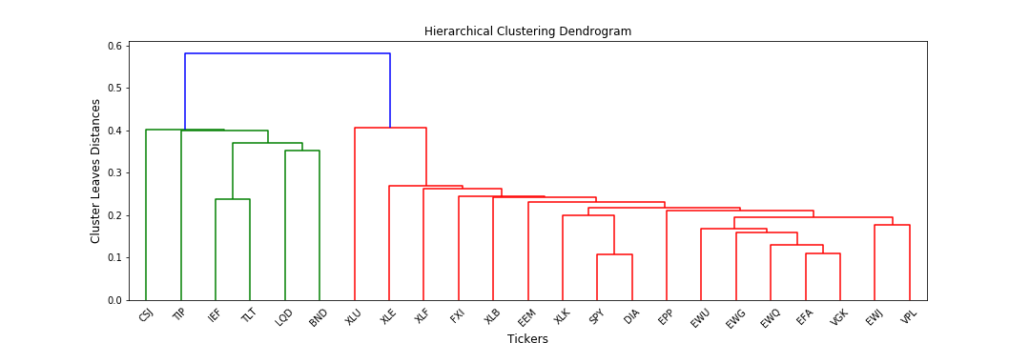
The hierarchical tree clustering algorithm identifies and segregates the assets in our portfolio into different clusters. At the end of the step, you are left with a tree which can be visualised in the form of a dendrogram, as shown below:

Starting with each asset being an individual cluster, the clustering algorithm uses something called linkage to determine how to combine the clusters. There are different linkage methods which can be used – single, ward, average and complete. HRP employs single linkage clustering which builds the tree based on the distance between the two closest points in these clusters. This results in a chaining effect and makes the tree very deep and wide, preventing any dense clusters from being formed and affecting the weight allocations.

This has been explained in detail in Dr. Papenbrock’s previously mentioned thesis through the following image:

The chaining effect of single linkage results in large weights to be allocated to few assets and an unequal distribution of the portfolio. Hence, using other linkage methods is important for optimal allocation – something which is incorporated in HERC. By default, it uses Ward linkage but users can specify any other methods to work with it.

Identifying the Optimal Number of Clusters

The hierarchical tree in the previous image starts with one big cluster and successively breaks into two new clusters at each level, with the end result being that each asset is in its own individual cluster. There are some problems with this approach:

Forming such large trees makes the algorithm computationally slow for very large datasets.
Letting the tree grow completely on our data also leads to the problem of overfitting. This can result in very small inaccuracies in the data leading to large estimation errors in the portfolio weights.

All these problems indicate a need to enforce an early stopping criteria for the tree and a way to calculate the exact number of clusters required. We will later talk about how this is handled by the HERC algorithm.

Not Following the Dendrogram Structure

During recursive bisection, the weights trickle down the tree until all the assets at the bottom-most level are assigned the respective weights. The problem here is that HRP does not stay true to the dendrogram structure, and instead it chooses to bisect the tree based on the number of assets.

Recursive Bisection Difference between Hierarchical Risk Parity and Hierarchical Equal Risk Contribution

The above figure is taken from HERC paper and illustrates the importance of following the tree structure. If you look closely, dividing the tree based on number of assets wrongly separates assets $\{1, 2\}$ and $\{3, 4\}$ while the correct cluster composition should have been $\{1\}$ and $\{2, 3, 4\}$ . Thomas Raffinot modified the recursive bisection of HRP to stay true to the natural dendrogram structure and we will later see how this affects the portfolio weights.

Variance as a Measure of Risk

In the recursive bisection step, HRP uses the variance of the clusters to calculate the weight allocations. This ensures that assets in clusters with minimum variance/volatility receive higher weights. We all know that estimates of risk in the form of the covariance matrix are always prone to errors and is one of the major factors why portfolio optimisation methods fail to perform in the real world. At the same time, even if we are able to obtain an almost-accurate estimate of the covariances of the assets, it is extremely sensitive to small changes in the market conditions and ultimately result in serious estimation errors.

Also, while variance is a very simple and popular representation of risk used in the investing world, it can underestimate the true risk of a portfolio which is why there are many other important risk metrics used by investment managers that can try to ascertain the true risk of a portfolio/asset. HERC modifies the recursive bisection of HRP to allow investors to use alternative risk measures – Expected Shortfall (CVaR), Conditional Drawdown at Risk (CDaR) and Standard Deviation. In Dr. Raffinot’s words:

Hierarchical Equal Risk Contribution portfolios based on downside risk measures achieve statistically better risk-adjusted performances, especially those based on the Conditional Drawdown at Risk.

Enter Hierarchical Equal Risk Contribution

Having understood the limitations of HRP, in this section, I will go over each of the steps of the HERC algorithm in a detailed manner.

Hierarchical Tree Clustering

This step breaks down the assets in our portfolio into different hierarchical clusters using the famous Hierarchical Tree Clustering algorithm. Specifically, we calculate the tree clusters based on the $TxN$ matrix of stock returns where $T$ represents the time-series of the data and $N$ represents the number of stocks in our portfolio. Note that this method combines the items into a cluster rather than breaking down a cluster into individual items i.e. it does an agglomerative clustering. Let’s understand how the clusters are formed in a step-by-step manner:

Given a $TxN$ matrix of stock returns, calculate the correlation of each stock’s returns with the other stocks which gives us an $NxN$ matrix of these correlations, ⍴
The correlation matrix is converted to a correlation-distance matrix $D$ , where,
\begin{aligned}
D(i, j) = \sqrt{0.5 * (1 – ⍴(i, j))}
\end{aligned}
Now, we calculate another distance matrix $\overline{D}$ where, \begin{aligned}
\overline{D}(i, j) = \sqrt{\sum_{k=1}^{N}(D(k, i) – D(k, j))^{2}}
\end{aligned}It is formed by taking the Euclidean distance between all the columns in a pair-wise manner.
A quick explanation regarding the difference between $D$ and $\overline{D}$ – for two assets $i$ and $j$ , $D(i, j)$ is the distance between the two assets while $\overline{D}(i, j)$ indicates the closeness in similarity of these assets with the rest of the portfolio. This becomes obvious when we look at the formula for calculating $\overline{D}$ – we sum over the squared difference of distances of $i$ and $j$ from the other stocks. Hence, a lower value means that assets $i$ and $j$ are similarly correlated with the other stocks in our portfolio.
We start forming clusters of assets using these distances in a recursive manner. Let us denote the set of clusters as $U$ . The first cluster $(i^{*}, j^{*})$ is calculated as, \begin{aligned}
U[1] = argmin_{(i,j)} \overline{D}(i, j)
\end{aligned}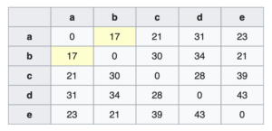 In the above figure, stocks $a$ and $b$ have the minimum distance value and so we combine these two into a cluster.
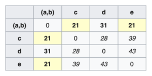
We now update the distance matrix $D$ by calculating the distances of other items from the newly formed cluster. This step is called linkage clustering and there are different ways of doing this. Hierarchical Risk Parity uses single linkage clustering which means the distances between two clusters is defined by a single element pair – those two elements which are closest to each other.
We remove the columns and rows corresponding to the new cluster – in this case we remove rows and columns for stocks $a$ and $b$ . For calculating the distance of an asset $i$ outside this cluster, we use the following formula \begin{aligned} \overline{D}(i, U[1]) = min( \overline{D}(i, a), \overline{D}(i, b) ) \end{aligned} Using the above formula we calculate distances for $c$ , $d$ and $e$ from cluster $(a, b)$ . \begin{aligned} \overline{D}(c, U[1]) = min( \overline{D}(c, a), \overline{D}(c, b) ) = min(21, 30) = 21\end{aligned}\begin{aligned} \overline{D}(d, U[1]) = min( \overline{D}(d, a), \overline{D}(d, b) ) = min(31, 34) = 31\end{aligned}\begin{aligned} \overline{D}(e, U[1]) = min( \overline{D}(e, a), \overline{D}(e, b) ) = min(23, 21) = 21\end{aligned}
In this way, we go on recursively combining assets into clusters and updating the distance matrix until we are left with one giant cluster of stocks as shown in the following image where we finally combine $d$ with $((a, b), c, e)$ .
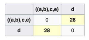
Finally, in hierarchical clustering, the clusters are always visualised in the form of a nice cluster diagram called dendrogram. Below is the image of the hierarchical clusters for our stock data,

Selecting the Optimal Number of Clusters

This is where HERC deviates from the traditional HRP algorithm. The first step grows the tree to its maximum depth and now it is time to prune it by selecting the required number of clusters. Dr. Raffinot has used the famous Gap Index method for this purpose. It was developed by Tibshirani et. al at Stanford University and is a widely used statistic in clustering applications.

Let’s say you have a data with $k$ clusters – $C_{1}, C_{2}, C_{3},....., C_{k}$ . Then the sum of pairwise distances for a cluster, $C_{r}$ is given by, \begin{aligned}D_{r} = \sum_{i, i^{/} \in C_r}d_{ii^{‘}} \end{aligned} where $d_{ii^{'}}$ is the Euclidean distance between two data points $i$ and $i^{'}$ . Based on this, the authors calculate the within-cluster sum of squares around the cluster means – $W_k$ (cluster inertia) \begin{aligned}W_k = \sum_{r = 1}^{k}\frac{D_{r}}{2n_{r}}\end{aligned} where $n_{r}$ is the number of data points in the $r^{th}$ cluster. Having calculated the cluster inertia, the Gap statistic is given by the following equation, \begin{aligned}Gap_{n}(k) = E^{*}_{n}[log(W_k)] \: – \: log(W_k)\end{aligned} where $E^{*}$ is an expectation from some reference distribution. According to the authors, the optimal value of clusters – $k^{*}$ – will be the one maximising $Gap_{n}(k)$ .

I will not go into the further details about the method and its mathematical motivations, but if you want to delve deeper, I highly suggest you read the original paper – Estimating the Number of Clusters in a Data Set via the Gap Statistic.

Pruning the hierarchical tree to the optimal number of clusters not only reduces overfitting but also helps achieve better weight allocations. The above image is taken from HERC paper and illustrates the importance of number of clusters on weight allocations.

Top-down Recursive Bisection

Having found the required number of clusters, this step calculates weights for each of them. Let us use the following diagram as a reference.

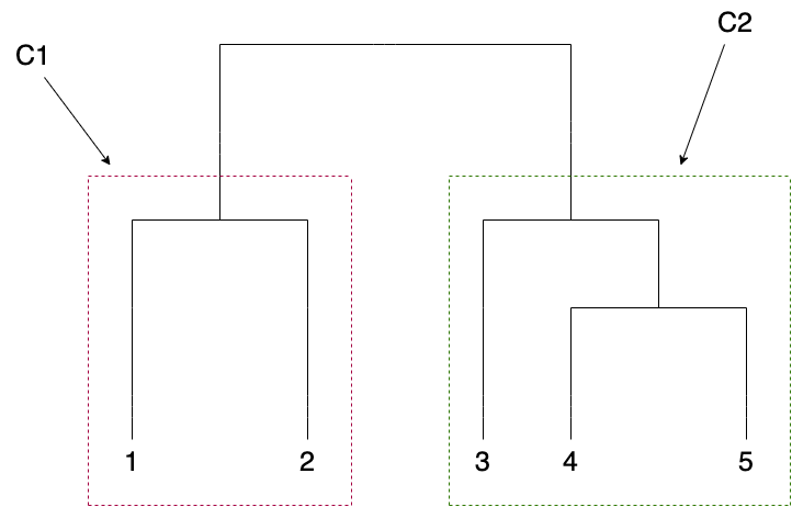
At the top of the tree, we have one big cluster and its weight is 1.
We now descend through the dendrogram structure and successively assign weights at each level of the tree. At each point, the tree always bisects into two sub-clusters, let’s say – $C_1$ and $C_2$ The respective cluster weights are given by the following formulae,\begin{aligned}CW_{C_1} = \frac{RC_{C_1}}{RC_{C_1} + RC_{C_2}}\end{aligned}\begin{aligned}CW_{C_2} = 1 \: – \: CW_{C_1}\end{aligned} $RC_{C_1}$ and $RC_{C_2}$ refers to the risk contribution of $C_1$ and $C_2$ respectively. Any traditional measure of risk can be used here and HERC currently supports the following ones – Variance, Standard Deviation, Expected Shortfall (CVaR) and Conditional Drawdown at Risk (CDaR). The $RC$ for a cluster is the additive risk contribution of all individual assets in that cluster. For example, from the above figure, if $C_1 = \{1, 2\}$ and $C_2 = \{3, 4, 5\}$ , then, \begin{aligned}RC_{C_1} = RC_1 + RC_2\end{aligned}\begin{aligned}RC_{C_2} = RC_3 + RC_4 + RC_5\end{aligned} where $RC_1$ is the risk associated with the $1^{st}$ asset and so on.
Recurse through the tree until all the clusters have been assigned weights.

Naive Risk Parity within Clusters

The last step is to calculate the final asset weights. Let us calculate the weights of assets residing in $C_2$ i.e. assets 3, 4 and 5.

The first step is to calculate the naive risk parity weights, $W_{NRP}$ , which uses the inverse-risk allocation to assign weights to assets in a cluster.\begin{aligned}W^{i}_{NRP} = \frac{\frac{1}{RC_i}}{\sum_{k=3}^{5}\frac{1}{RC_k}}, i \in \{3, 4, 5\}\end{aligned}
Multiply the risk parity weights of assets with the weight of the cluster in which they reside.\begin{aligned}W^{i}_{final} = W^{i}_{NRP} \: * \: CW_{C_2}, i \in \{3, 4, 5\}\end{aligned}

In this way, the final weights are calculated for assets in all the other clusters.

A Quick Comparison of HRP and HERC

If you are reading this section, then you have already made it through the difficult parts of the article and all that is left is to see the algorithm in action. In this section, I will do a quick comparison of the differences between HRP and HERC by running both the algorithms on real asset data and observing the respective weight allocations. I will be using PortfolioLab’s HERC implementation for this example.

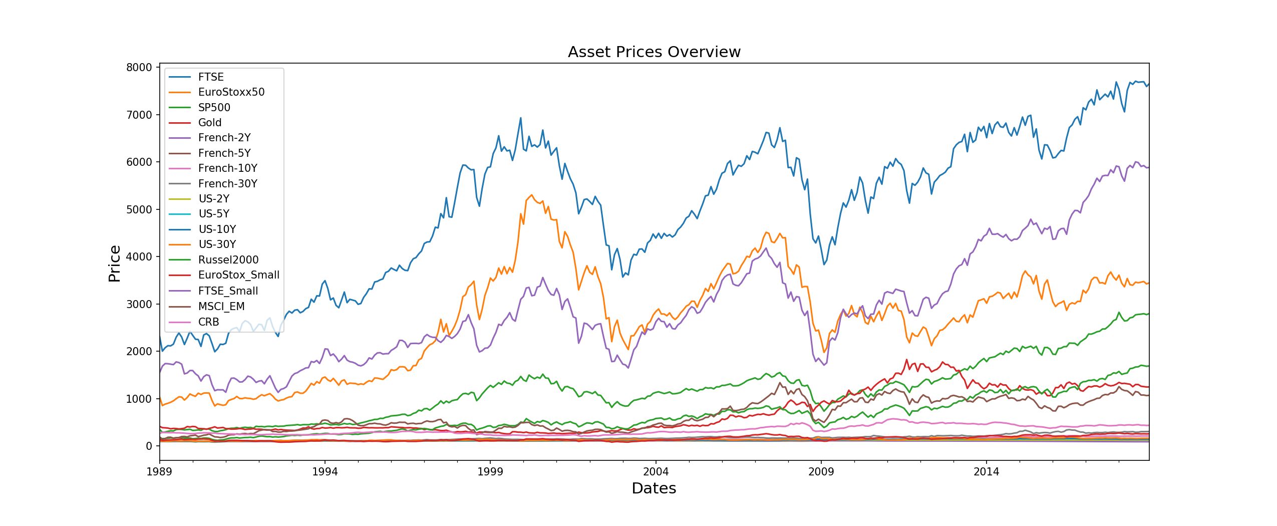
We will be using a multi-asset dataset of 17 assets from different asset classes (bonds and commodities) and exhibiting different risk-return characteristics.

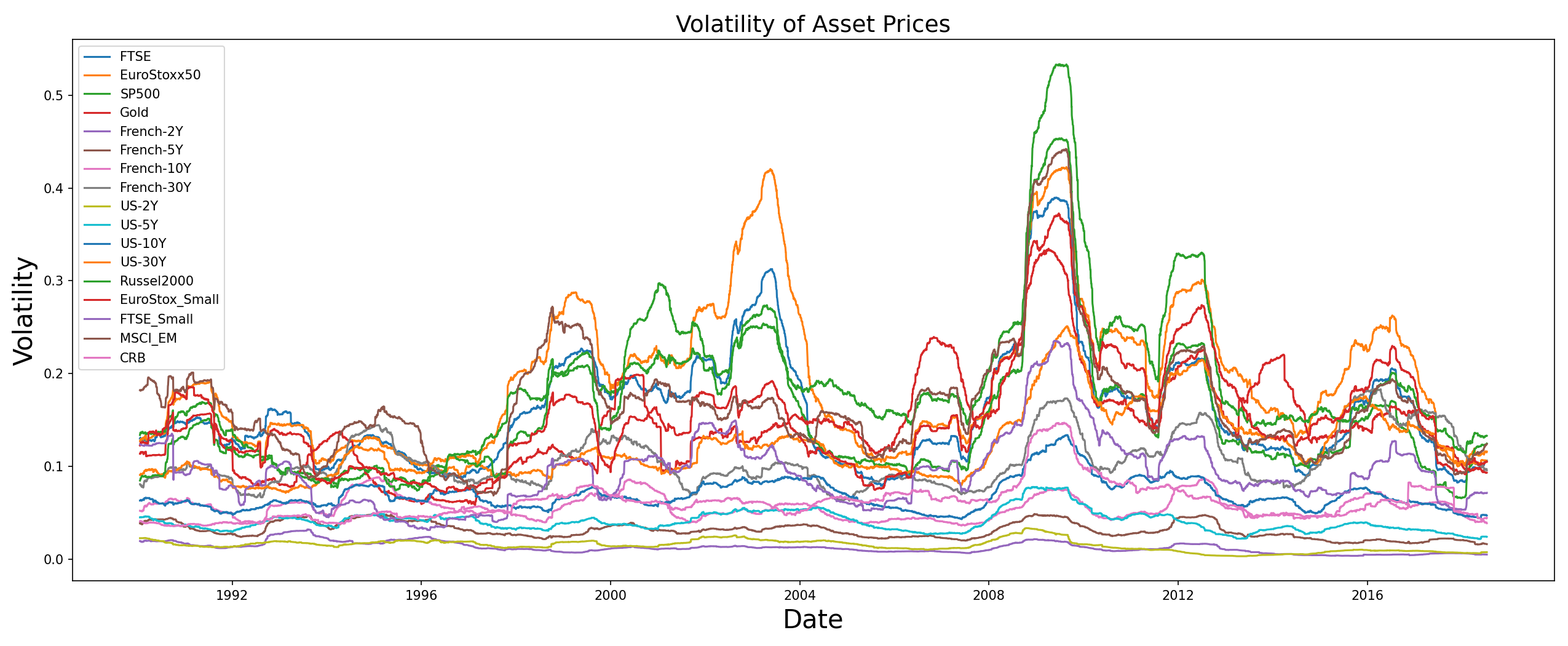
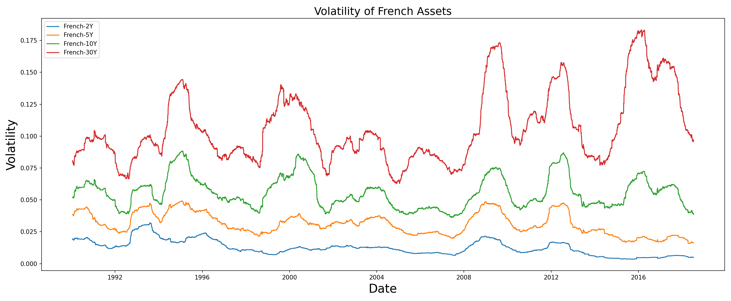
We also give a quick look at the volatilities of these assets,

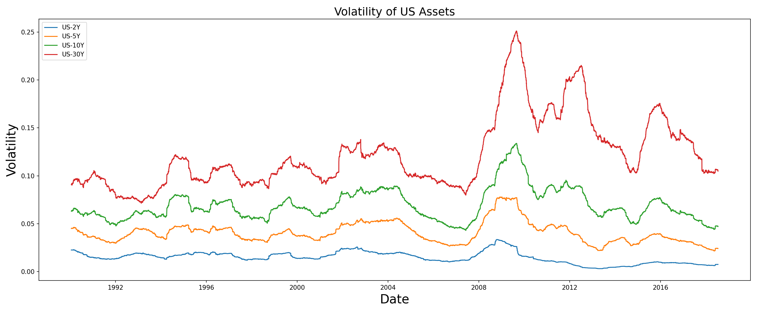
In particular let us focus on the volatilities of the US and French bonds,

HERC Equal Weighting vs HRP

In his paper, Dr. Raffinot concludes with the following statement – “Hierarchical 1/N is very difficult to beat”. Apart from the different risk measures mentioned earlier, HERC can also allocate using the equal weighting metric where the risk is allocated equally among assets in the clusters. Here I have compared HERC’s equal weighting allocations with those of HRP’s minimum variance. By default, HERC uses Ward clustering (which is what Raffinot has used in his paper) and HRP employs the single linkage clustering.

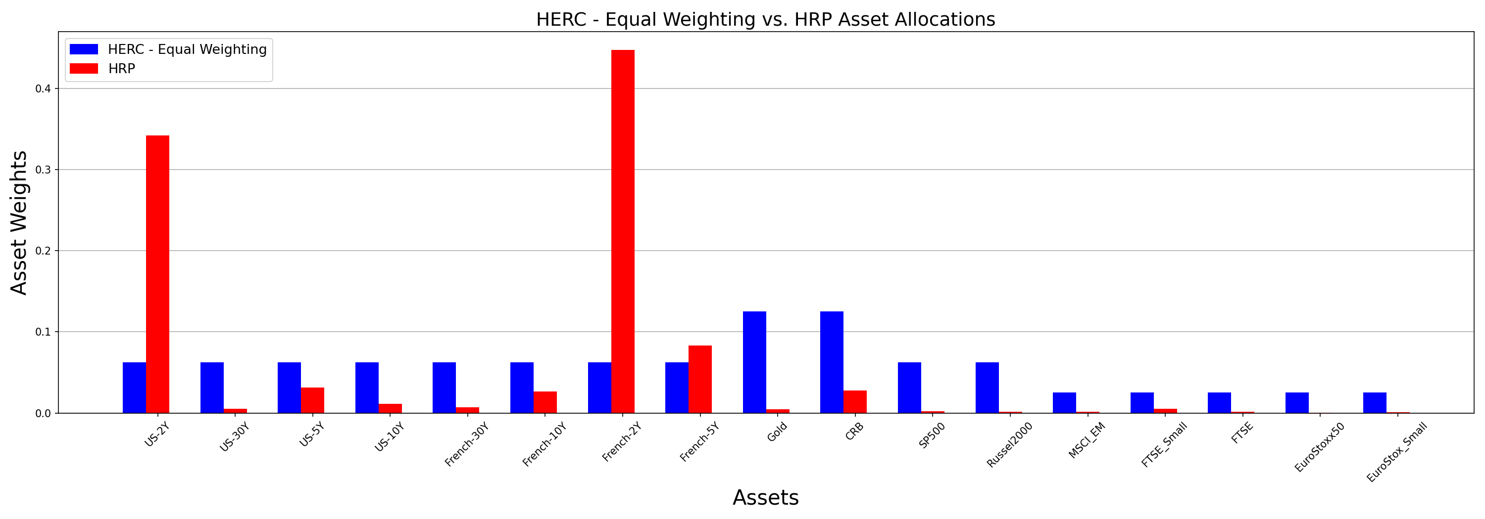
HRP has allocated most of the weights to US-2Y and French-2Y because these bonds exhibit the least amount of volatility (look at the plot of volatilities). However, the other assets have received lower weights and one can say that the HRP portfolio is sparsely distributed.
On the other hand, HERC allocated weights equally to all the assets in a cluster. All US bonds, being part of the same cluster, got the same weights and this is true for French bonds too (except French-2Y). Although similar to traditional equal weight portfolios, a major difference in HERC’s equal weighting scheme is that only the assets in a cluster compete for these allocations. Instead of all the 17 assets receiving equal weights, the weights are divided unequally among the clusters and then divided equally within them. This ensures that the portfolio remains well diversified by assigned weights to all assets and at the same time making sure that only items within a cluster compete for these allocations.

HERC Minimum Variance vs HRP

In the following comparison, I will change HERC’s risk measure to variance. All other parameters stay the same.

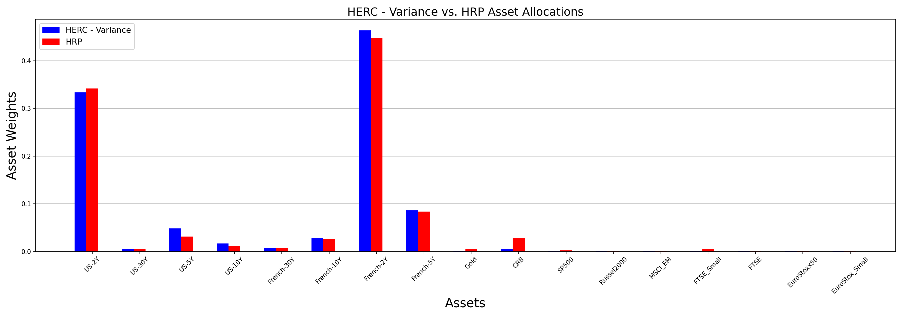While the HRP portfolio remains unchanged, the HERC weights undergo a significant change and are more in sync with the former. You can observe that it has increased the weights for US and French bonds, while decreasing allocations for other assets. Furthermore, there are slight differences between both the portfolios – HERC decreases the weight of US-2Y and spreads it across the cluster to the other US assets. At the same time, it slightly increased the allocation for French-2Y asset as compared to the HRP one.

Note that this was a very rudimentary comparison of these two algorithms and in no way a final one. For an in-depth analysis, one should resort to more statistically adjusted methods like Monte Carlo simulations, generating bootstrapped samples of time-series returns etc… However, the purpose of this section was to provide a quick glimpse of how small differences in the working of these algorithms affect the final portfolios generated by them.

Conclusion and Further Reading

By building upon the notion of hierarchy introduced by Hierarchical Risk Parity and enhancing the machine learning approach of Hierarchical Clustering based Asset allocation, the Hierarchical Equal Risk Contribution aims at diversifying capital and risk allocation. Selection of appropriate number of clusters and the addition of different risk measures like CVaR and CDaR help in generating better risk-adjusted portfolios with good out-of-sample performance. In my opinion this algorithm is an important addition to the growing list of hierarchical clustering based allocation strategies.

The following links provide a more detailed exploration of the algorithms for further reading.