By Ruth du Toit

Exploring Mean Reversion and Momentum Strategies in Arbitrage Trading

Our recent reading group examined mean reversion and momentum strategies, drawing insights from the article, “Dynamically combining mean reversion and momentum investment strategies” by James Velissaris. The aim of the paper was to create a diversified arbitrage approach that combines mean reversion and momentum strategies to exploit the strengths of both strategies.

Mean reversion and momentum strategies have distinct characteristics. Mean reversion strategies centre around stocks reverting to their mean values and capitalising on relative mispricing among stocks. In contrast, momentum strategies focus on stocks that have shown strong recent performance and are expected to continue that trend.

Set-Up

The dataset for the study is made up of an in-sample period from November 1, 2005, to October 31, 2007 which includes the Quant Quake of August 2007, and an out-of-sample period from November 1, 2007, to October 30, 2009 which includes the Global Financial Crisis of 2008. For the mean reversion model, daily closing price data from the S&P 500 index were utilised whereas the momentum strategy incorporated daily closing price data sourced from Bloomberg for ten different stock market indices.

Inspired by Avellaneda and Lee’s work on ‘Statistical Arbitrage in the U.S. Equities Markets’, the equity mean reversion model aimed to maintain a market-neutral position. However, its failure to meet this primary objective casts doubt on the model’s overall effectiveness. Furthermore, Quadratic programming was employed for portfolio rebalancing, focusing on optimising asset allocation.

In-Sample Performance

In the article, the mean reversion strategies proved to be highly effective within the in-sample environment (although this shouldn’t be surprising). 

Mean reversion outperforming momentum in-sample

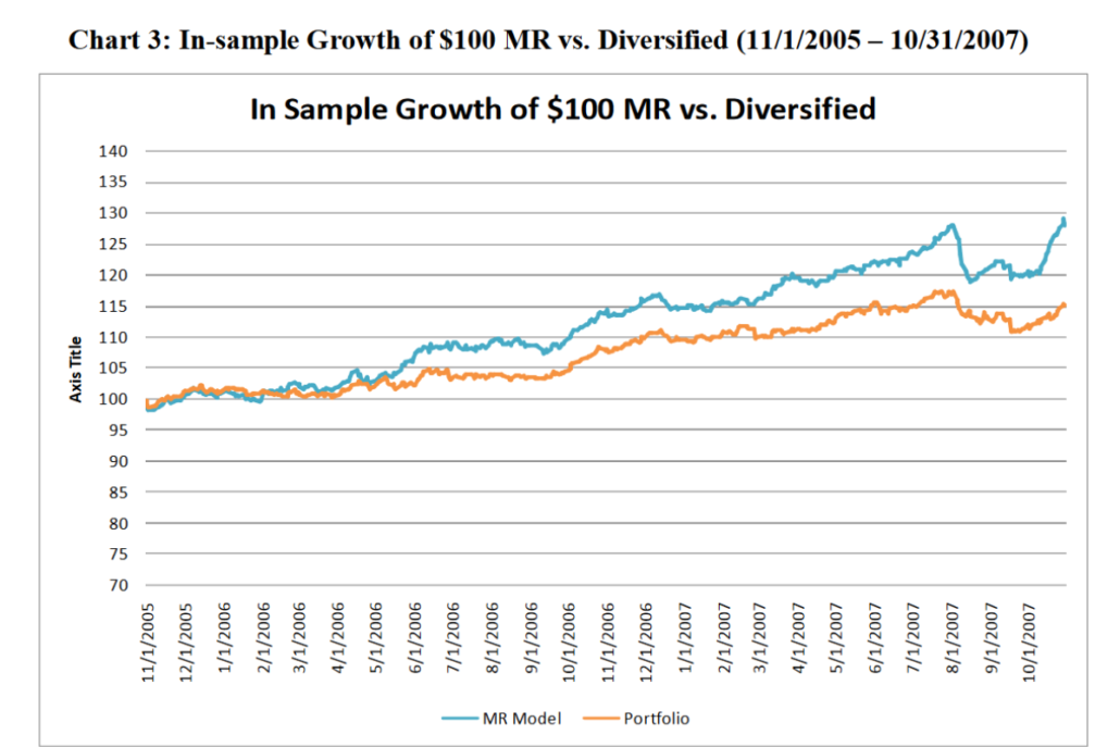
The problem with in-sample results

Mean reversion’s apparent effectiveness at the in-sample dataset is based on the use of historical market knowledge and parameter optimisation to align with past data. However, it’s important to be sceptical of in-sample data, and to approach out-of-sample performance expectations with caution, as historical predictability may not necessarily translate to future periods. 

In the reading group, we discussed possible ways to improve the generalization of our mean reversion strategies to the out-of-sample dataset. Can techniques such as regularisation or cross-validation offer a solution?

Addressing these challenges is important to ensure the robustness of trading strategies when they are used in real-world scenarios. While in-sample performance provides some value, it’s the out-of-sample testing that validates the strategy’s adaptability to changing market conditions. Ultimately, however, what really matters is trading the strategy with real money in a live trading environment.

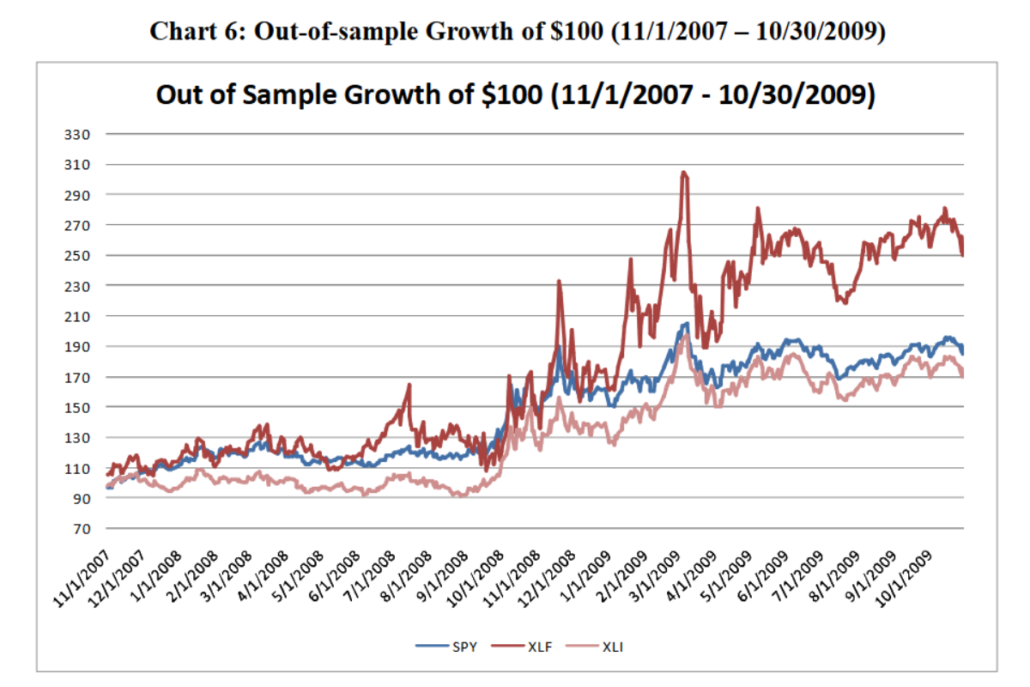
Out-of-Sample Performance

Momentum, as a strategy, relies on recent price trends, which tend, but are not guaranteed, to continue for longer periods in real markets. 

Near the end of the 2008 global financial crisis, Momentum strategies seem to have been effective. Note, however, that the fact that this strategy performed well at the end of 2008 suggests that it may have been capitalising on a potential market recovery during that period.

Momentum’s out-of-sample performance

Market Neutral vs. Hedging Opportunities

While the mean reversion model aspired to a market-neutral stance, it consistently fell short of this target in practice. Although we could  argue it could act as a hedge during broader market downturns, according to the paper we might be better off remaining sceptical. Thus, it would be premature to regard mean reversion as a foolproof method for reducing overall risk exposure through low-correlation strategies.

Directions in Trading Strategies

In-sample, mean reversion demonstrates its effectiveness, raising important questions about its adaptability in out-of-sample scenarios. Can the tools such as regularisation and cross-validation help address this challenge? Meanwhile, the Momentum strategy excels in the real world, emphasising the importance of adaptability in our trading approach.

This discussion also serves as a reminder that trading isn’t only about beating the market, it’s also about managing risk. 

Stay tuned for further analysis and strategic insights as Hudson & Thames continues to navigate the field of quantitative finance.

For more information about our H&T reading group visit: https://hudsonthames.org/reading-group/

A group of strategies, named statistical arbitrage or pairs trading strategies are well-known for being market-neutral gained their popularity among institutional and individual investors. In general, to develop a pairs trading strategy, one needs to figure out two aspects, the first is how to select assets to form a process with mean-reverting properties, and the second is how to decide when and how to trade such process. In recent years, many methods have been proposed to answer these two questions. Fitting the spread to an O-U process, cointegration tests, and stochastic control methods are commonly used but are theoretically complicated. For the most part, the trading strategies constructed using these approaches aim to exploit the mean-reverting nature of the constructed spread.

Traditional pairs trading strategies are prone to failures when fundamental or economic reasons cause a structural break and the pair of assets that were expected to move together are no longer having a strong relationship. Such a break may result in asset price spread having abnormally high deviations failing to revert to its historical mean values. Under these circumstances, betting on the spread to revert to its historical mean would result in a loss. To overcome the problem of detecting whether the deviations are temporary or longer-lasting, Bock, M. and Mestel, R. (2009) bridge the literature on Markov regime-switching models and the scientific work on statistical arbitrage to develop a set of useful trading rules for pairs trading.

Pairs trading or statistical arbitrage is a famous strategy among institutional and individual investors since the 1990s. The concept behind this kind of strategy is straightforward. If the prices of assets move together historically, this tendency is likely to continue in the future. When the spread of the prices diverges from its long-term mean, one can short sell the over-priced stock, buy the under-priced one, and wait for the spread to converge to take the profit.

In general, to develop a pairs trading strategy, we need to solve two major issues, the first is how to select assets to form a process with mean reversion properties, and the second is how to decide when to trade…

The hedge ratio estimation problem is one of the most important issues for portfolio managers.

The hedge ratio estimation methods can be divided into two:
– Single Period Method
– Multi-Period Method

In this blog post, we’ll simply go through the main concepts of each method and closely follow a paper by Lopez de Prado, M.M. and Leinweber, D. (2012). Advances in Cointegration and Subset Correlation Hedging Methods. Therefore, for further details and implementation, we would highly recommend you to read individual papers for each of the methods provided.

This is a series where we aim to cover in detail various aspects of the classic Ornstein-Uhlenbeck (OU) model and the Ornstein-Uhlenbeck Jump (OUJ) model, with applications focusing on mean-reverting spread modeling under the context of pairs trading or statistical arbitrage. Given the universality and popularity of those models, the techniques discussed can easily be applied to other areas where the OU or OUJ model seems fit.

In this article, we aim to dive into the classic OU model, and illustrate the most common tasks encountered in applications:

1. How to generate an OU process.
2. Caveats in fitting an OU process.

In our previous article, we’ve discussed a couple of trading strategies exploiting arbitrage between similar stocks using stochastic optimal control methods. A major shortcoming of those approaches is that we restricted ourselves to constructing delta-neutral portfolios. Along with this, the ratio between the stocks in the portfolio is fixed at the start of the investment timeline. These assumptions make the problem simpler, as we only need to calculate the portfolio weights for the spread process as a whole. But, this approach, as [Liu and Timmermann (2013)] discusses, is suboptimal. In this article, we will be discussing a generalized approach that allows the weights corresponding to the stocks in the portfolio to move freely, along with looking at the shortcomings of the previous approaches.

We have discussed Basic Distance Approach in the previous blog post. In this post, we’ll look into one of the advanced methods in the Distance Approach and its differences to the Basic Distance Approach. If you haven’t read the previous blog post, we recommend reading it before you read this post.

So, what is the Pearson Correlation Approach? It is a type of Distance Approach and applies Pearson correlation on return level for identifying pairs. The main concept is similar to the Basic Distance Approach, where pairs are formed with a particular rule, and a portfolio is constructed based on the trading signals of pairs.

There are many types of approaches you can use in pairs trading, but the Distance Approach is one of the most widely used because of its simplicity. The basic concept is as follows: Using Euclidean squared distance on the normalized price time series, n closest pairs of assets are chosen as pairs.

Then, with selected pairs, if the difference between the price of elements in a pair diverged by more than a threshold(ex. 2 standard deviations), the positions are opened. We have a long position for a stock with a lower price and a short position for a higher price in the portfolio.

Pairs selection is the first crucial step to building a pairs trading strategy. And it is no surprise, to perform it correctly, one must diligently examine, compare and contrast numerous test results, graphs and characteristics. For example, cointegration analysis alone can be performed in one of two methods – utilizing the Engle-Granger approach or the Johansen approach. To truly have the complete picture of the pairs suitability, with the Engle-Granger approach, the researcher should perform the test(and further analysis) for both possible combinations, A/B or B/A, in a pair since it is sensitive to which asset we choose to be the “dependent” one.
The Johansen test, in turn, provides multiple cointegration vectors, which also should be examined separately and taken into account. Not to mention the possible analysis of the residuals, auto-correlation tests, etc., brings even more data to the table for you to make your judgement.

And now, we have two options: memorize everything or constantly switch between numerous parameters and plots to check, contrast and compare. It results in loading your brain with tons of ‘noise’ that distracts from focusing on the evaluation itself. But it doesn’t have to be this way. Data analysis thrives when there is order, accessibility and clarity. And what embodies these three qualities better than combining everything into an interactive well-rounded tear sheet?