Extended Optimal Arbitrage Strategies
by Vijay Nadimpalli
Join the Reading Group and Community: Stay up to date with the latest developments in Financial Machine Learning!
Introduction
In our previous article, we’ve discussed a couple of trading strategies exploiting arbitrage between similar stocks using stochastic optimal control methods. A major shortcoming of those approaches is that we restricted ourselves to constructing delta-neutral portfolios. Along with this, the ratio between the stocks in the portfolio is fixed at the start of the investment timeline. These assumptions make the problem simpler, as we only need to calculate the portfolio weights for the spread process as a whole. But, this approach, as [Liu and Timmermann (2013)] discusses, is suboptimal. In this article, we will be discussing a generalized approach that allows the weights corresponding to the stocks in the portfolio to move freely, along with looking at the shortcomings of the previous approaches.
As you might know, in a typical convergence trade, two assets trade at different prices but have the same (or similar) payoff with certainty at a future date. Familiar examples of convergence trades are merger arbitrage (risk arbitrage) and pairs trading (relative value trades). The strategies for these types of trades conventionally consider taking positions of equal size but opposite signs either in portfolio weight or in the number of shares(delta-neutrality). Although this consideration seems intuitive at first, as any future risks are offset between the pair of stocks, such strategies will typically not be optimal. These delta-neutral convergence trades do not exploit the short-run risk-return tradeoff as they are built to work on long-term arbitrage opportunities.
Some convergence traders close out their position when prices converge, and in some cases, the price difference between two assets in a convergence trade will disappear permanently after it reaches zero. To model these strategies, [Liu and Timmermann (2013)] look at a stopped cointegration process whereby asset prices follow a cointegrated process before the difference reaches zero and the difference remains at zero afterwards.
We will be looking at two types of strategies in this article.
- Optimal Portfolio Strategy
- Continuous cointegration process
- Stopped cointegration process
- Delta Neutral Portfolio Strategy
- Continuous cointegration process
- Stopped cointegration process
The optimal portfolio strategy is unconstrained, without any delta neutrality conditions which limit mispricing exploitation. Delta neutral portfolio strategy, as the name suggests, calculates the portfolio weights with the delta neutrality condition. And for each of these strategies, we also look at both the continuous cointegration process and the stopped cointegration process.
The setup
Before we dive into the various strategies in detail, let’s start looking at the setup of the problem. In this paper, the authors model risky arbitrages under the assumption that individual asset prices contain a random walk component, but that pairs of asset prices can be cointegrated. This model captures the presence of a mean-reverting mispricing component that reverts to zero in the long run. This is a fairly standard assumption that lets us calculate closed-form solutions in some cases. We’ll look at when closed-form solutions exist later in the article. Also, this assumption gives us a mean-reverting error correction term [Engle and Granger (1987)] denoted by ![]() . It is calculated as the difference in the log prices between the two assets. Some of the important features of
. It is calculated as the difference in the log prices between the two assets. Some of the important features of ![]() is that,
is that,
- It represents the expected excess return above the risk premium implies by CAPM.
- It’s expected value is zero in the long run.
- time variation of
 let’s model both:
- Absolute mispricing – abnormal expected returns over the CAPM benchmark values.
- Relative mispricing – relative prices of the two assets.
An interesting point about xt is it lets us model both the absolute mispricing(abnormal expected returns over the CAPM), which dominates at short time periods, and the relative mispricing(relative prices of the two assets), which plays a key role in longer periods as the price differences can be expected to revert to zero and the optimal portfolio is long in the (relatively) underpriced asset and short in the (relatively) overpriced asset. We will explain how ![]() can be used to model these mispricings later.
can be used to model these mispricings later.
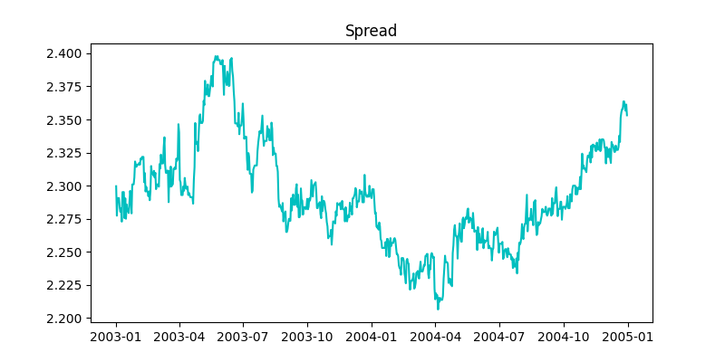
Fig. 1: Spread ![]() for the Shell-Royal Dutch pair.
for the Shell-Royal Dutch pair.
Key Assumptions of the model:
- Riskless asset paying a rate of return
 .
. - Market index
 which follows a geometric random walk.

where the market risk premium,
 , and market volatility,
  , are both constant, and
  is a standard Brownian motion.
 - The pricing errors in the model is denoted by
 . Yes, this is the mean-reverting error correction term discussed before.

- The two risky assets
 and
and  are given by,

where
 ,
,  ,
,  ,
,  , and
, and  are constant parameters.
  and
and  are standard Brownian motions, and
  ,
,  , and
, and  are all mutually independent for
  .
.  , a very important assumption that I will be explaining later.
Understanding these equations
The evolutions of the risky assets given above might seem complex and strange at first, so let us explain the intuition behind it.
The cointegration setup assumed in this model captures the feature that two assets with identical payoffs can trade at different prices. Let us give an example. The shares of Shell and Royal-Dutch traded at different prices before their unification in 2005, even though they represent the same underlying assets. The cointegration setup used above perfectly represents this scenario. If the time of convergence of the two prices was known with certainty, there would be a riskless arbitrage opportunity and investors would have shorted the overpriced stock in the same amount as they would have been long in the underpriced stock. In reality, however, although the two stock prices can be expected to converge over time, the date at which this would occur is not known before, and so this is an example of risky arbitrage. To model the above risky arbitrage, it is standard to assume that idiosyncratic risks are independent across different stocks with the market risk representing the only source of correlation among different assets.
In this case, both assets are claims on similar fundamentals and so the presence of common idiosyncratic risk, ![]() , is to be expected. The two asset prices are correlated both because of their exposure to the same market-wide risk factor (
, is to be expected. The two asset prices are correlated both because of their exposure to the same market-wide risk factor (![]() ) and common idiosyncratic risk (
) and common idiosyncratic risk (![]() ) but also because of the mean-reverting error correction term (
) but also because of the mean-reverting error correction term (![]() ), which will induce correlation between the two asset prices even in the absence of the two former components.
), which will induce correlation between the two asset prices even in the absence of the two former components.
Alpha and absolute mispricing
You might be wondering what those ![]() parameters in the price dynamics represent. These parameters along with the
parameters in the price dynamics represent. These parameters along with the ![]() term showcase the mispricing “alphas”, or put it simply, they represent the amount by which each asset is overpriced or underpriced relative to CAPM. This is also called the absolute mispricing of the asset.
term showcase the mispricing “alphas”, or put it simply, they represent the amount by which each asset is overpriced or underpriced relative to CAPM. This is also called the absolute mispricing of the asset.
Let me form some intuition about how this came to be. Let’s look at the expected return of asset 1. This is given by the equation ![]() . Let’s suppose that
. Let’s suppose that ![]() . Here, the expected returns of the assets satisfy the CAPM relation,
. Here, the expected returns of the assets satisfy the CAPM relation, ![]() . This means that essentially both assets are fairly priced and there is no mispricing to exploit. Not interested in this case, are we? Let’s look at a scenario that we are actually interested in.
. This means that essentially both assets are fairly priced and there is no mispricing to exploit. Not interested in this case, are we? Let’s look at a scenario that we are actually interested in.
Suppose the ![]() ‘s are nonzero. When
‘s are nonzero. When ![]() , asset one has a higher expected return than is suggested by the CAPM relation, that is it has a positive alpha, and that implies that asset one is underpriced. Conversely, when
, asset one has a higher expected return than is suggested by the CAPM relation, that is it has a positive alpha, and that implies that asset one is underpriced. Conversely, when ![]() asset one has a lower expected return than justified by its risk, that is it has a negative alpha and therefore is overpriced. Similarly, when
asset one has a lower expected return than justified by its risk, that is it has a negative alpha and therefore is overpriced. Similarly, when ![]() , asset two has a positive alpha and thus is underpriced; when
, asset two has a positive alpha and thus is underpriced; when ![]() , asset two has a negative alpha and is overpriced. I hope that this clears up the reasoning behind the term mispricing “alphas”.
, asset two has a negative alpha and is overpriced. I hope that this clears up the reasoning behind the term mispricing “alphas”.
Cointegration and relative mispricing
Let us explain briefly about relative mispricing and how it can be modeled by ![]() , which as we have seen before is the difference in the logarithm of the prices of two assets. To keep the mispricing between the two assets stationary and the pricing errors “small” compared with either of the price processes,
, which as we have seen before is the difference in the logarithm of the prices of two assets. To keep the mispricing between the two assets stationary and the pricing errors “small” compared with either of the price processes, ![]() is modeled as a mean-reverting process. Mean reversion in
is modeled as a mean-reverting process. Mean reversion in ![]() captures the temporary nature of any mispricing.
captures the temporary nature of any mispricing.
![]()
![]()
A very important assumption we made earlier is that ![]() . This is necessary to make the rate of mean reversion of the OU process defining
. This is necessary to make the rate of mean reversion of the OU process defining ![]() positive, which ensures that
positive, which ensures that ![]() is mean-reverting.
is mean-reverting.
To sum up, absolute mispricing is determined in the short run by the conditional alphas, whereas relative mispricing is determined in the long run by cointegration between asset prices.
Cases to consider
In this article, we will be discussing two cases of arbitrage opportunities,
- recurring arbitrage opportunities
- nonrecurring arbitrage opportunities
In the first case, ![]() only spends an extremely short time at zero, and it is represented at all times by the OU process with zero long-run mean. We will be able to derive a closed-form solution for the portfolio weights in this case. Coming to the second case, any price difference gets permanently eliminated the first time
only spends an extremely short time at zero, and it is represented at all times by the OU process with zero long-run mean. We will be able to derive a closed-form solution for the portfolio weights in this case. Coming to the second case, any price difference gets permanently eliminated the first time ![]() touches zero. Investors are expected to close out all positions at this point. Unfortunately, finding a closed-form solution is not feasible in this case, so we rely on numerical methods to calculate the resulting PDE from the HJB equation.
touches zero. Investors are expected to close out all positions at this point. Unfortunately, finding a closed-form solution is not feasible in this case, so we rely on numerical methods to calculate the resulting PDE from the HJB equation.
Portfolio Construction
Let’s move on to looking at the important details where we focus on building an optimal portfolio. Our portfolio consists of a risk-free asset, the market portfolio weighted by ![]() and the two risky assets weighted by
and the two risky assets weighted by ![]() and
and ![]() respectively. The dynamics of the total wealth of the portfolio are given by,
respectively. The dynamics of the total wealth of the portfolio are given by,
![]()
Next, we look at investor preferences and choose a utility function to model the investor. Here, the authors assume that the investor maximizes the expected value of a power utility function defined over terminal wealth, ![]()
The investor’s value function is given by
![]()
where ![]() is the wealth at time
is the wealth at time ![]() obtained by the optimal trading strategy.
obtained by the optimal trading strategy.
Using this value function, we can start calculating the HJB equation and the optimal portfolio weights.
Unconstrained Optimal Strategies
Continuous cointegration
For the continuous cointegrated price process (recurring arbitrage opportunities), we get a closed-form solution for the optimal portfolio weights.
The optimal weights on the market portfolio, ![]() , and the individual assets,
, and the individual assets, ![]() , are given by
, are given by

Stopped Cointegration
Next, consider the case in which the price difference, ![]() , stays at zero when it reaches zero so that it follows a “stopped” cointegrated process. This case is relevant for “one-shot” arbitrages, such as risk arbitrage in mergers and acquisitions. Alternatively, if the investor decides to close out the position once prices converge, we can also view the price process as a stopped cointegrated process.
, stays at zero when it reaches zero so that it follows a “stopped” cointegrated process. This case is relevant for “one-shot” arbitrages, such as risk arbitrage in mergers and acquisitions. Alternatively, if the investor decides to close out the position once prices converge, we can also view the price process as a stopped cointegrated process.
In this case, there is no closed-form solution for the value function, but we can solve for it numerically and obtain the optimal portfolio weights.
Delta-Neutral strategies
The delta-neutrality condition is usually assumed in many studies of convergence trades. For example, [Jurek and Yang (2007)] and [Mudchanatonsuk (2008)] both assume that ![]() . As mentioned before, although the market-neutral strategy is very popular, it can be suboptimal. The best way to actually achieve a delta-neutral position is to use the market index to hedge away the market exposure in the mispriced assets. Using only the mispriced assets to achieve delta-neutrality will necessarily under-exploit opportunities offered by mispricing in the individual stocks.
. As mentioned before, although the market-neutral strategy is very popular, it can be suboptimal. The best way to actually achieve a delta-neutral position is to use the market index to hedge away the market exposure in the mispriced assets. Using only the mispriced assets to achieve delta-neutrality will necessarily under-exploit opportunities offered by mispricing in the individual stocks.
Continuous cointegration
For the continuing cointegrated price process (recurring arbitrage opportunities), we get a closed-form solutions for the optimal portfolio weights.

where ![]() . An interesting thing to note here is that the portfolio weights for the market index do not vary with time.
. An interesting thing to note here is that the portfolio weights for the market index do not vary with time.
For the stopped cointegration case, we can solve the PDE numerically as there is no closed-form solution.
The optimal strategy is delta-neutral if ![]() .
.
An interesting point here is that different combinations of the ![]() and
and ![]() parameters are likely to reflect the (relative) liquidity of the two assets. For example, if two high-volume stocks are both traded in liquid markets, it’s likely that their prices adjust equally rapidly, and so
parameters are likely to reflect the (relative) liquidity of the two assets. For example, if two high-volume stocks are both traded in liquid markets, it’s likely that their prices adjust equally rapidly, and so ![]() holds as a good approximation. A good point in case is the Royal Dutch and Shell shares traded on the Amsterdam and London stock exchanges, for which both
holds as a good approximation. A good point in case is the Royal Dutch and Shell shares traded on the Amsterdam and London stock exchanges, for which both ![]() ’s are nearly equal, as we see will see in the results.
’s are nearly equal, as we see will see in the results.
Results
In this section, I will look at the results obtained from trading these strategies on the Shell-Royal Dutch pair of stocks.
Data from 1994 to 2004 is considered for running these backtests and the evaluation period is 2 years. To start, the training data is inputted to the fit method, which calculates the estimates for the parameters of the model.
# Importing required modules
import pandas as pd
from arbitragelab.stochastic_control_approach import OptimalConvergence

# Loading up the data
data = pd.read_csv('shell-rdp-close_USD.csv', index_col='Date').ffill()
data.index = pd.to_datetime(data.index, format="%d/%m/%Y")
data_train_dataframe = data['1994':'2002']
data_test_dataframe = data['2003':'2004']

# Creating a class object
oc = OptimalConvergence()

# Calling the fit method to estimate the parameters
oc.fit(data_train_dataframe, r = 0.05, mu_m = 0.20, sigma_m = 0.3)
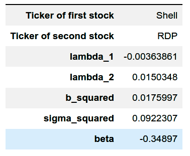
Fig. 2: Estimated Parameters for the Shell-Royal Dutch pair.
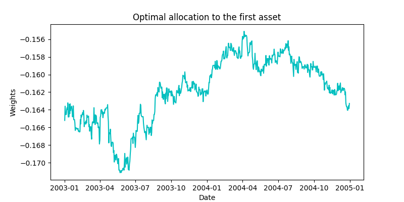
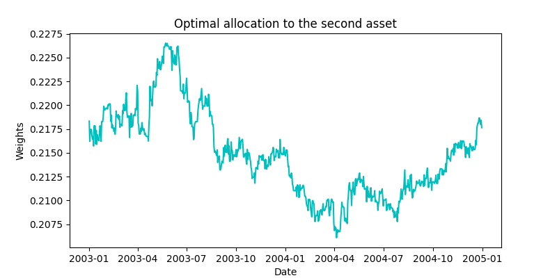
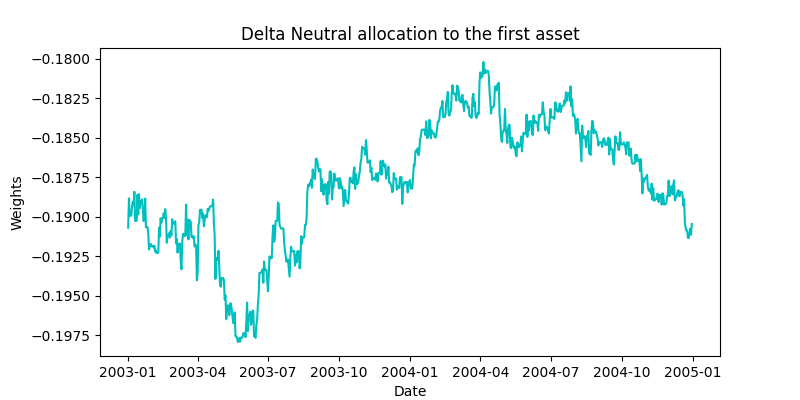
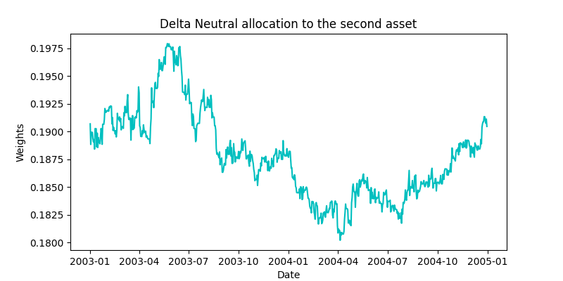
Now to calculate the portfolio weights, we make use of the evaluation data along with some user-inputted parameters, which are inputted to the corresponding portfolio_weights methods. These methods will calculate the corresponding weights for the three assets in our portfolio. The gamma parameter inputted to these methods signifies the risk aversion characteristics of an investor. The higher the value of gamma, the more risk averse the investor is.
# Calculating the optimal weights
phi_1, phi_2, phi_m = oc.unconstrained_portfolio_weights_continuous(data_test_dataframe, gamma=4)

# Calculating the delta-neutral weights
phi_1, phi_2, phi_m = oc.delta_neutral_portfolio_weights_continuous(data_test_dataframe, gamma=4)
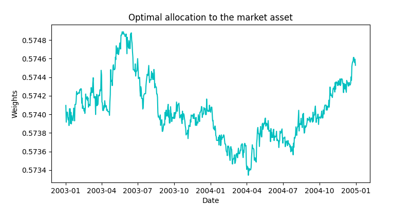
Fig. 3: Optimal Portfolio Weights for the market asset.
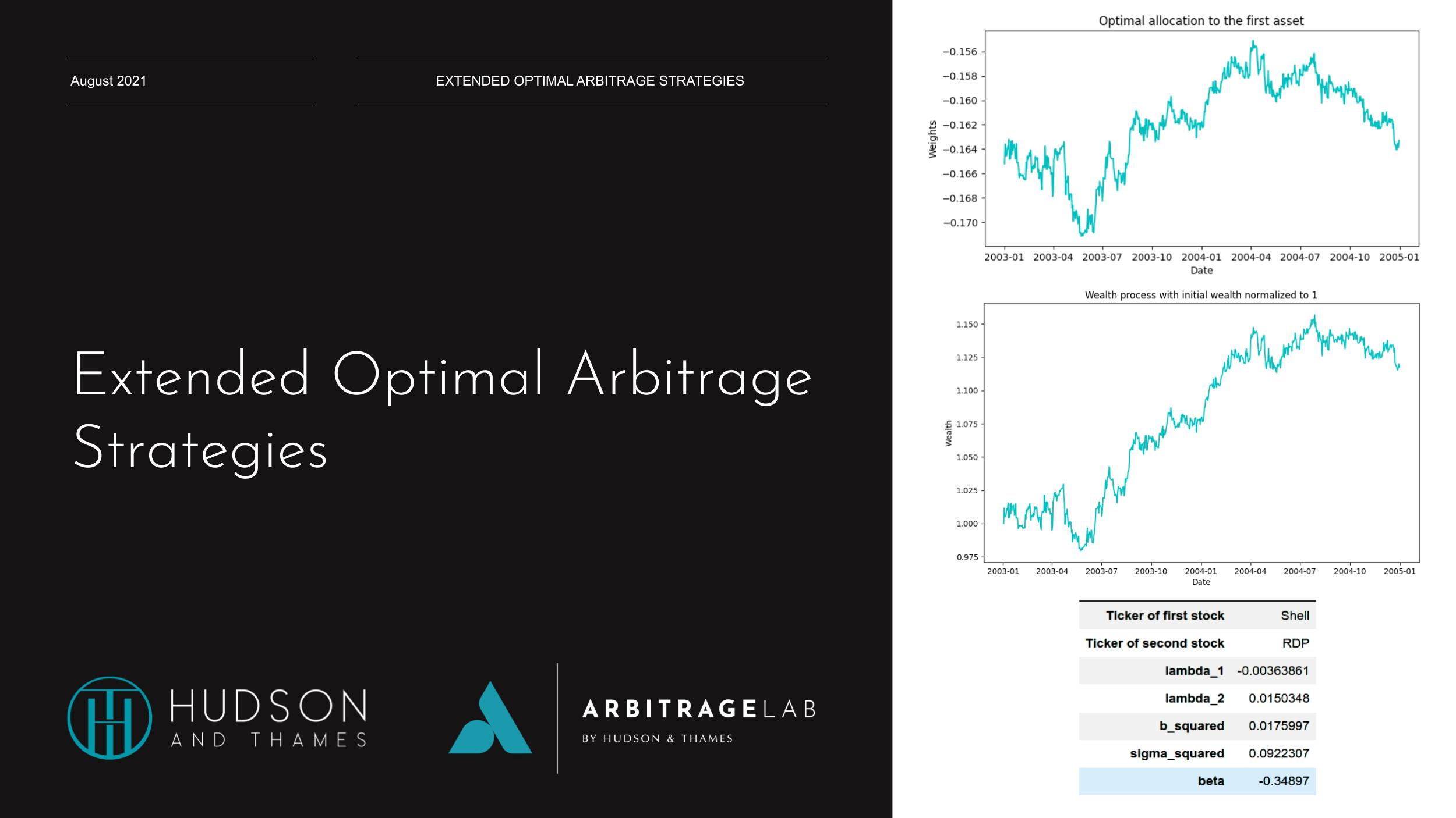
The figures given above show the unconstrained optimal allocation to the Shell and Royal Dutch assets in our portfolio along with the market asset. Figures below show the delta-neutral portfolio allocations to the two Shell and Royal Dutch assets.
An interesting thing to note here is that the portfolio weights in the two sets of plots move similarly to each other. If we look at the values of the estimated ![]() ‘s shown in the above figure,
‘s shown in the above figure, ![]() and
and ![]() . As I mentioned previously, if
. As I mentioned previously, if ![]() and
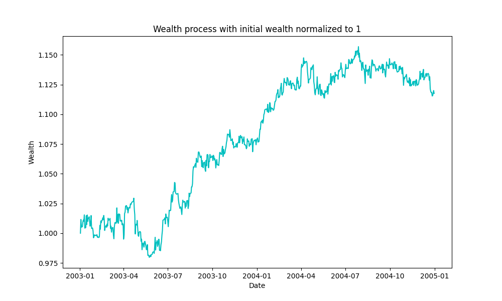
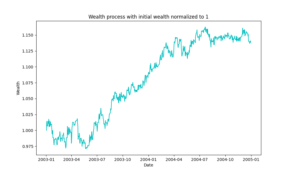
and ![]() are pretty close to each other, both the strategies start to give similar results. The same can be seen in the total wealth plots for the two strategies given below. Although there are some drawdowns, both the strategies were able to generate a decent profit.
are pretty close to each other, both the strategies start to give similar results. The same can be seen in the total wealth plots for the two strategies given below. Although there are some drawdowns, both the strategies were able to generate a decent profit.
Fig. 4: Total wealth of the portfolio in the delta-neutral portfolio strategy.
Fig. 5: Total wealth of the portfolio in the optimal portfolio strategy.
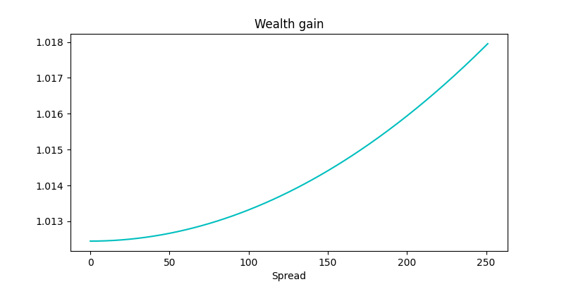
Excess wealth gain
Finally, let’s look at the excess wealth gain that can be achieved by using the optimal portfolio weights instead of the delta-neutral portfolio weights, which reveals some interesting results. To calculate the above plot, we assume that ![]() . So the
. So the ![]() values are quite different from each other.
values are quite different from each other.
# Excess wealth gain from using the optimal weights model
R = oc.wealth_gain_continuous(gamma=4)
Fig. 6: Expected wealth gains as a function of the spread ![]() .
.
As can be seen from the plot above, the unconstrained optimal portfolio starts to generate quite a bit more profit in comparison to the delta neutral portfolio, especially as the spread between the two assets increases.
Comments
Convergence trades form an important part of relative value trading strategies. The model presented in this article, argues that taking a delta-neutral trading strategy might not be optimal, as by allowing the weights corresponding to the assets to move freely, the strategy not only incorporates the arbitrage opportunity but also diversification benefits. This model relies on daily rebalancing and so produces high transaction costs. A comparison with a less active trading rule, such as in the Gatev (2006) paper, would provide better insights on how this model fares in light of actual market frictions.
Check out our lecture on the topic:
References
- Gatev, Evan, William N. Goetzmann, and K. Geert Rouwenhorst, 2006, Pairs Trading: Performance of a Relative Value Arbitrage Rule, Review of Financial Studies, 19, 797-827.
- Jurek, J.W. and Yang, H., 2007, April. Dynamic portfolio selection in arbitrage. In EFA 2006 Meetings Paper.
- Krauss, C., 2017. Statistical arbitrage pairs trading strategies: Review and outlook. Journal of Economic Surveys, 31(2), pp.513-545.
- Liu, J. and Timmermann, A., 2013. Optimal convergence trade strategies. The Review of Financial Studies, 26(4), pp.1048-1086.
- Mudchanatongsuk, S., Primbs, J.A. and Wong, W., 2008, June. Optimal pairs trading: A stochastic control approach. In 2008 American control conference (pp. 1035-1039). IEEE.

