Introducing Online Portfolio Selection

By Alex Kwon

Join the Reading Group and Community: Stay up to date with the latest developments in Financial Machine Learning!

Online Portfolio Selection is an algorithmic trading strategy that sequentially allocates capital among a group of assets to maximize the final returns of the investment.

Traditional theories for portfolio selection, such as Markowitz’s Modern Portfolio Theory, optimize the balance between the portfolio’s risks and returns. However, OLPS is founded on the capital growth theory, which solely focuses on maximizing the returns of the current portfolio.

Through these walkthroughs of different portfolio selection strategies, we hope to introduce a set of different selection tools available for everyone. Most of the works will be based on Dr. Bin Li and Dr. Steven Hoi’s book, Online Portfolio Selection: Principles and Algorithms, and further recent papers will be implemented to assist the development and understanding of these unique portfolio selection strategies.

The package and module behind this implementation are currently in the works and will be published on PortfolioLab soon.

Problem Formulation

Price:
- Asset $i$ ‘s price at time $t$ is $p_{t,i}$ .
Price Relative:
- Ratio of the current time’s price to the last time’s price.
- Asset $i$ ‘s price relative at time $t$ is $x_{t,i}$ .
Portfolio Weight:
- Represent the allocation of capital to a particular asset.
- Assume that the weights are non-negative and that the sum of the weights is one, which will simulate a long-only, no leverage environment.
Portfolio Return:
- Cumulative product of all previous returns.
- $S_0$ represents the initial capital, and each product of price relative and portfolio weights represent the increase in capital for a particular time period.

Data

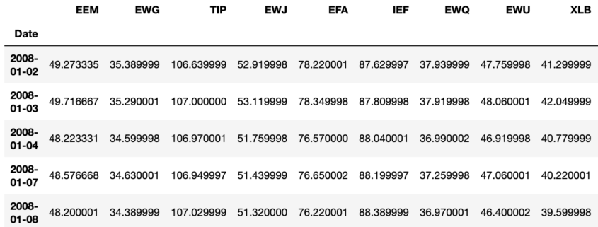
We will use the ETF data included in the PortfolioLab library for analysis. This includes 23 ETF’s with closing prices from 2008 to 2016.

Buy and Hold

Buy and Hold is a strategy where an investor invests in an initial portfolio and never rebalances it. The portfolio weights, however, change as time goes by because the underlying assets change in prices.

Returns for Buy and Hold can be calculated by multiplying the initial weight and the cumulative product of relative returns.

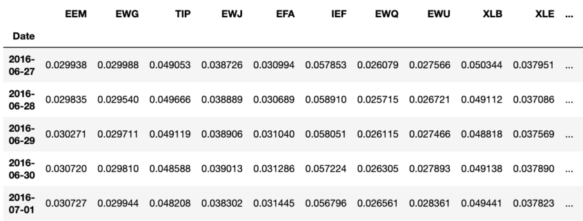
$S_n(BAH(b_1)) = b_1 \cdot \left(\overset{n}{\underset{t=1}{\bigodot}} x_t\right)$

Because we didn’t specify a weight when we allocated to the strategy, initial weights are uniformly distributed across all the ETFs for time 0.

The weights change over time because the ETF prices fluctuate.

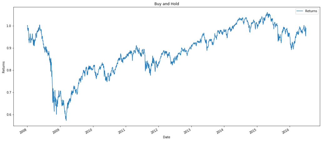
With the crash in 2009, Buy and Hold strategies have returned almost the same returns from the initial allocation. The results would vary depending on the weights of stock. Generally, this strategy is a great starting point as a benchmark comparison, because we can compare the historical performances of active and passive investing.

Best Stock

Best Stock strategy chooses the best performing asset in hindsight.

The best performing asset is determined with an argmax equation stated below. The portfolio selection strategy searches for the asset that increases the most in the price for the given time period.

$b_0 = \underset{b \in \Delta_m}{\arg\max} \: b \cdot \left(\overset{n}{\underset{t=1}{\bigodot}} x_t \right)$

Once the initial portfolio has been determined, the final weights can be represented as buying and holding the initial weight.

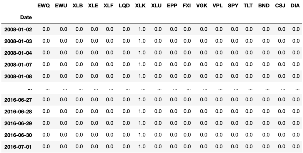
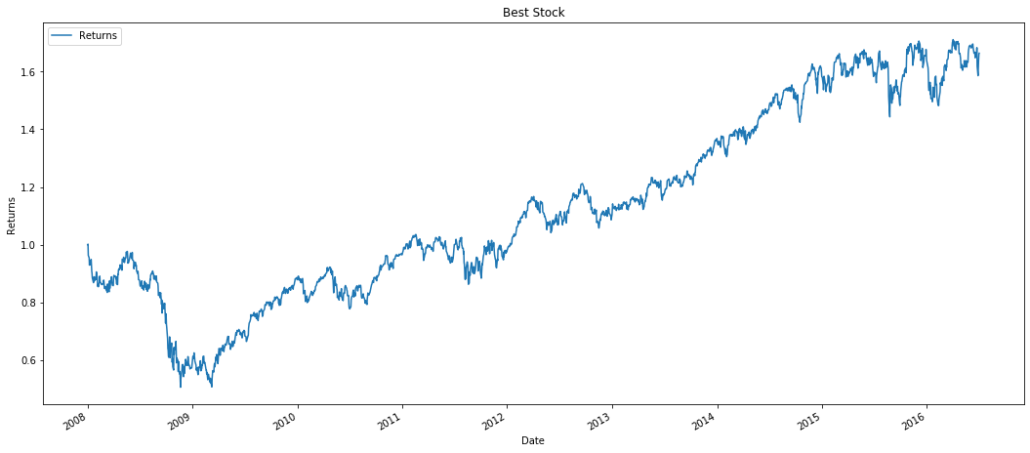
$S_n(BEST) = \underset{b \in \Delta_m}{\max} b \cdot \left(\overset{n}{\underset{t=1}{\bigodot}} x_t \right) = S_n(BAH(b_0))$

If we examine all of the weights assigned to best stock, we notice that all the weights are set to 0 except for XLK. For the given period and price data, XLK was the best performing asset, so the portfolio strategy chooses to allocate all of its own weight on XLK.

As seen with the above graph, we are directly tracking XLK, the best performing ETF during this period. The same exact graph can be replicated by buying only XLK from the beginning using the Buy and Hold strategy since we are not rebalancing the portfolio.

Constant Rebalanced Portfolio

Constant Rebalanced Portfolio rebalances to a certain portfolio weight every time period. This particular weight can be set by the user, and if there are no inputs, it will automatically allocate equal weights to all assets. The total returns for a CRP can be calculated by taking the cumulative product of the weight and relative returns matrix.

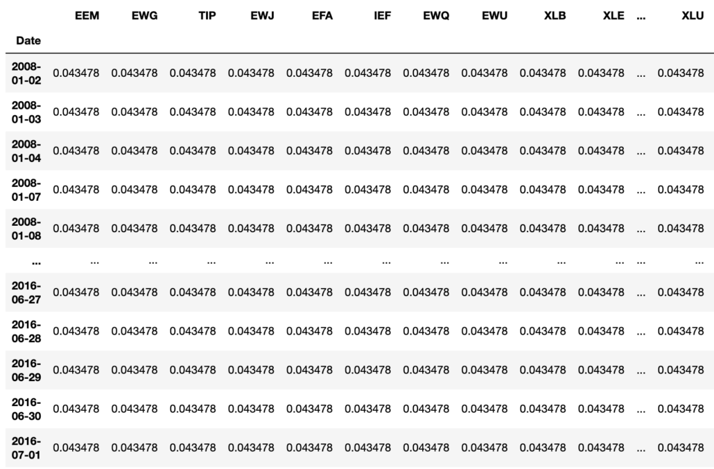
$S_n(CRP(b)) = \overset{n}{\underset{t=1}{\prod}} \: b^{\top}x_t$

This particular CRP is called a Uniform CRP because it starts with uniform weights, and we can see that the weights stay constant over the given time period.

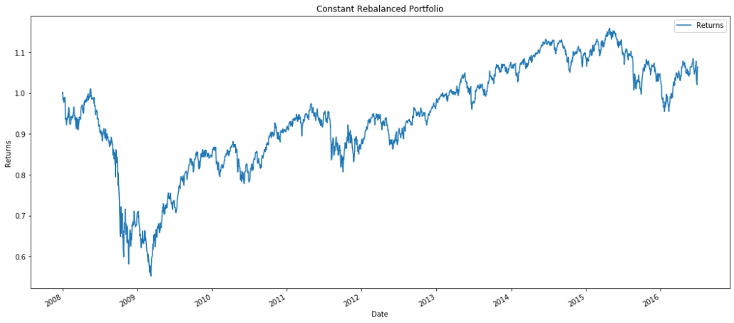
In a way, CRP performs a passive mean reversion. For the assets that decrease in prices, it’s corresponding weights for the following period should decrease. However, by allocating weights to even out and return to the predetermined number, the portfolio consistently shifts weights from increasing assets to decreasing assets. The returns for CRP is actually very similar to the Buy and Hold strategy that we saw earlier.

For this particular set of assets, UCRP was a suboptimal strategy. Although we are consistently rebalancing our portfolio to account for price changes, it was unable to take advantage of the fluctuating market dynamics. If we account for transaction costs, the returns would be lower than an ordinary Buy and Hold.

Best Constant Rebalanced Portfolio

Best Constant Rebalanced Portfolio is a strategy that is implemented in hindsight. It uses the same weight for all time periods. However, it determines these weights by having the complete market sequence of the past. The objective function for BCRP looks to maximize portfolio returns with the equation below.

$b^{\bf{\star}} = \underset{b^n \in \Delta_m}{\arg\max} \: S_n(CRP(b)) = \underset{b \in \Delta_m}{\arg\max} \overset{n}{\underset{t=1}{\prod}} \: b^{\top}x_t$

Once the optimal weight has been determined, the final returns can be calculated by using the CRP returns equation.

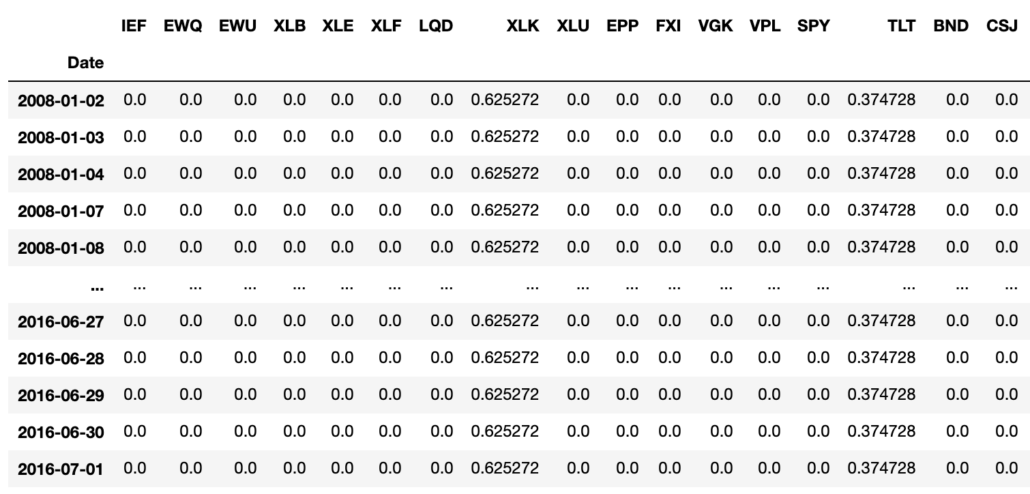
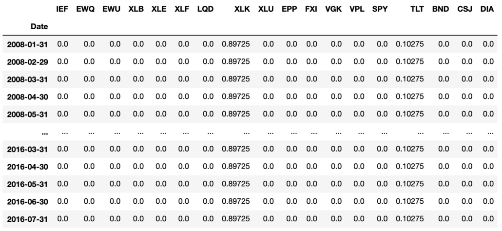
$S_n(BCRP) = \underset{b \in \Delta_m}{\max} \: S_n(CRP(b)) = S_n(CRP(b^{\bf \star}))$

The weights are the same from the beginning to the end. BCRP returns weights of 0.625272 to XLK, which was the best performing ETF, and 0.374728 to TLT, the second-best performing ETF.

Interestingly, TLT tracks US Treasury bonds of 20+ years and XLK tracks the S&P 500 technology sector. The portfolio weights returned by BCRP is the inverse of the popularized 60/40 portfolio of equity to bonds. For the assets of this dataset, there is a strong indication of a passive mean reversion with these two assets that allow the BCRP to produce returns that are higher than the Best Stock of XLK.

BCRP achieves higher returns than any other portfolio that we have seen so far. However, this is primarily due to the fact that we had the data of the complete market sequence. This is impossible to implement in the real market, but it is a good benchmark to keep in hand as we implement other strategies. For other portfolios and the given dataset, we should look to perform better than the 1.8 given with BCRP strategy.

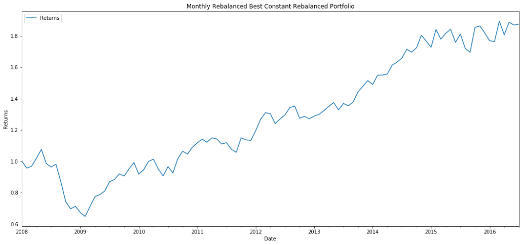
On another note, our strategies can be resampled to a given time period if we want to simulate a portfolio manager’s monthly rebalancing or if we want to minimize our transaction costs. We’ll examine a case where we monthly rebalance our portfolio.

The weights have changed to 0.89725 of XLK and 0.10275 TLT as we are now resampling on a monthly basis.

The graph is smoother compared to the daily rebalanced portfolio, and we actually achieve higher returns than the daily rebalanced one by a marginal amount. The monthly rebalancing most likely reduces market noise and follows the traditional mean reversion method to account for higher returns.

Conclusion

Through this post, we were able to explore the basic functionalities of PortfolioLab’s newest Online Portfolio Selection module. Readers were exposed to a basic introduction to the OLPS Benchmarks and will be able to replicate results using the simple methods of the new module.

The next notebook will focus on Momentum.

If you enjoyed reading this please leave us a star on GitHub and join our Slack channel to ask us any questions!

Online Portfolio Selection Strategies

Throughout the next couple of weeks, we will be releasing notebooks on the following strategies

Benchmarks
- Buy and Hold
- Best Stock
- Constant Rebalanced Portfolio
- Best Constant Rebalanced Portfolio
Momentum
- Exponential Gradient
- Follow the Leader
- Follow the Regularized Leader
Mean Reversion
- Anti-Correlation
- Passive Aggressive Mean Reversion
- Online Moving Average Reversion
- Robust Median Mean Reversion
Pattern Matching
- Nonparametric Histogram/Kernel-Based/Nearest Neighbor Log-Optimal
- Correlation Driven Nonparametric Learning
- Nonparametric Kernel-Based Semi-Log-Optimal/Markowitz/GV
Meta Algorithm
- Aggregating Algorithm
- Fast Universalization Algorithm
- Online Gradient Updates
- Online Newton Updates
- Follow the Leading History
Universal Portfolio
- Universal Portfolio
- CORN-U
- CORN-K
- SCORN-K
- FCORN-K