Why Model with Copula?

Well, essentially you just want to know how the two legs are “related”, and then exploit the structure for profit. Copula, a concept that enables mathematicians to analyze the dependency structure from multiple random variables, is an ideal superhero that is specifically tailored to deal with this problem. Just to name a few advantages:

1. It separates the marginal distributions from studying their “relation”, so you don’t need to worry about taking into account all the possible combinations of possible types of univariate distributions, greatly simplifying the amounts of code needed.
2. You can tune the dependency structure to your own liking, especially the tail dependencies. No more linear dependence assumptions telling you some events that happen yearly should occur every 10 billion years.
3. You can work with multiple stocks in a cohort, instead of just a pair, to create the ultimate trading unit for capturing mispricing in a much higher dimension.
4. Being a relatively novel approach, the playground for copula (especially the higher dimensional stuff) is much less crowded compared to other common quant strategies like vanilla distance and cointegration. This daunting Latin word, let’s be fair, scares a lot of people away.

Copula means “link” in Latin (And strictly speaking, its plural is copulae, but I will use copulas here, because I am an applied mathematician and have never used fancy stuff like lemmata or copulae for my writing). The key idea lies in modeling the relation between two random variables’ quantiles to avoid involving idiosyncratic marginal distributions.

Throughout this article, I will guide you through the important facts related to copula, with an applicative mindset, without digging too much into the bog of various mathematical analysis. This article is a definitive, conglomerate collection of important concepts regarding copula collected and derived from multiple journals and textbooks, so it has a lot of formulas and is not meant to be read line-by-line in one go, but as an article one can refer to for resources. We assume a generic understanding of applied probability and statistics. The fitting algorithms, sampling and exact trading strategies are separated for their own dedicated articles to keep the length manageable.

Those are the topics I aim to cover:

1. What is a bivariate copula and how to understand it?
2. What is tail dependence and why it is crucial for pairs trading?
3. What are Archimedean copulas and Elliptical copulas and how to understand a mixed copula?
4. Features (mostly tail dependence) of common copulas related to modeling pairs trading.
5. Interesting open problems to consider.

However, if you are still keen on the math side of those, I highly recommend going through the seminal book for a thorough analyst approach: An Introduction to Copulas by Professor Roger Nelsen.

Also, we limit our discussion to bivariate copulas unless clarified otherwise to avoid swimming in notations.

An Example

First, let’s start by doing the following calculations to try to temporarily bypass the mathematical definition, which may not help much unless we have an idea of where the copula comes from. Essentially we are just making the Q-Q (quantile-quantile) plot of two continuous random variables. Here is the process:

1. For two continuous random variables with fixed distributions, find their own marginal CDFs (cumulative density functions).
2. Sample from the two-random-variable pair multiple times.
3. Map the random samples into their quantile domain by their CDFs, you should get two uniformly distributed quantiles data in .
4. Plot the pair’s quantile-quantile data.

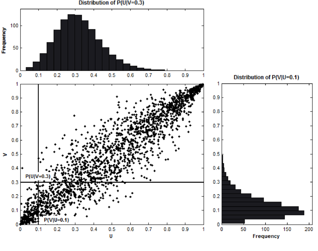
The picture below illustrates our construction well:

Fig. 1. An illustration of the conditional distribution function of V for a given value of U and the conditional distribution function of U for a given value of V using the N14 copula dependence structure. An example from “Trading strategies with copulas.” by Stander, Yolanda, Daniël Marais, and Ilse Botha.

A few points here to clarify: First, knowing the marginal distribution does not in any way determine this Q-Q plot at all, and this Q-Q plot tells the full dependency structure between the two random variables, it tells us how they are “related”. Second, we just plotted the samples from a copula according to its copula density , which is generally denoted as . The denser the dots, the higher the copula density. It is still not the copula itself because copula is the joint cumulative density of quantiles , and is defined in the next section. . Much like when you try to plot a univariate distribution, you sample from its CDF by generating uniformly from to plot its PDF, we are doing the same thing but in 2 dimensions.

Basic Concepts

Sklar’s Theorem

This definition is a natural abstraction of our sampling procedure above.

(Definition using Sklar’s Theorem) For two random variables , . and have their own fixed, continuous CDFs . Consider their (cumulative) joint distribution . Now take the uniformly distributed quantile random variable , , for every pair drawn from the pair’s quantile we define the bivariate copula as:

\begin{alignat*}{2}
C(u_1, u_2) &= P(U_1 \le u_1, U_2 \le u_2) \\
&= P(S_1 \le F_1^{-1}(u_1), S_2 \le F_2^{-1}(u_2)) \\
&= H(F_1^{-1}(u_1), F_2^{-1}(u_2)),
\end{alignat*}

where and are quasi-inverses of the marginal CDFs and . Let’s emphasize that copula is just the joint cumulative density for quantiles of a pair of random variables, do not get scared by its fancy Latin name. (I know it is a lot of symbols and there are more incoming, and if it is the first time for you to see this it might take a moment to wrap your head around all the material. It took me a few days to fully absorb this material. But trust me this theorem is the only part of the whole journey for one to know by heart for applications. For other materials in this article you only need to know them qualitatively and know where the formulas are when required.)

Sklar’s theorem guarantees the existence and uniqueness of a copula for two continuous random variables, clearing the way for the wonderful world of applications. Imagine what the world would be if you have to worry about its existence and uniqueness every time you use it, ughhhh!

Formal Definition

The following widely used formal definition focuses on the joint distribution (of quantiles) aspect of a copula.

(Formal Definition of Copula) A two-dimensional copula is a function where

such that

– (C1) and for all ;
– (C2) is 2-increasing, i.e., for with and :

\begin{alignat*}{2}
V_c \left( [a,b]\times[c,d] \right) := C(b, d) – C(a, d) – C(b, c) + C(a, c) \ge 0.
\end{alignat*}

Keep in mind that the definition of copula is just the joint cumulative density on quantiles of each marginal random variable, i.e.,

\begin{alignat*}{2}
C(u_1, u_2) = \mathbb{P}(U_1 \le u_1, U_2 \le u_2).
\end{alignat*}

And (C1)(C2) naturally comes from joint CDF: (C1) is quite obvious, and (C2) is just the definition of

\begin{alignat*}{2}
\mathbb{P}(a \le U_1 \le b, c \le U_2 \le d).
\end{alignat*}

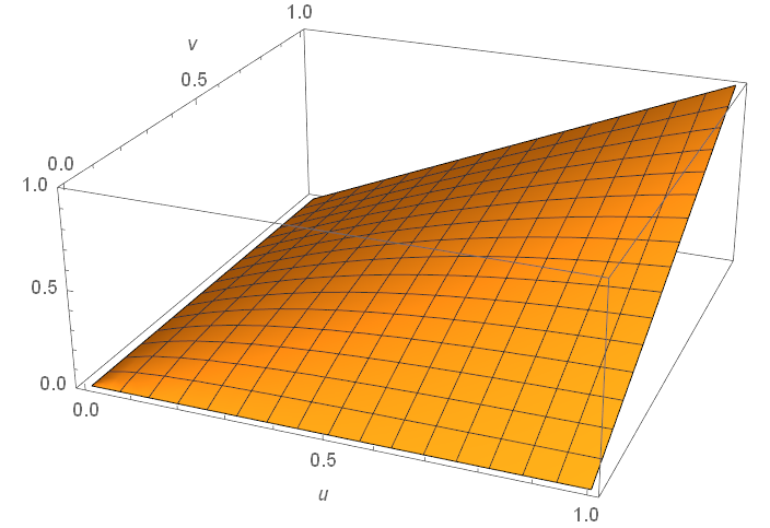
Fig. 2. Plot of for an N13 copula.

Related Concepts

We define the (cumulative) conditional probabilities:

\begin{alignat*}{2}
P(U_1\le u_1 | U_2 = u_2) &:= \frac{\partial C(u_1, u_2)}{\partial u_2}, \\
P(U_2\le u_2 | U_1 = u_1) &:= \frac{\partial C(u_1, u_2)}{\partial u_1},
\end{alignat*}

and the copula density :
\begin{alignat*}{2}
c(u_1 , u_2) := \frac{\partial^2 C(u_1, u_2)}{\partial u_1 \partial u_2},
\end{alignat*}
which by definition is the probability density. Those two concepts are crucial for fitting a copula to data and its application in pairs trading, and we do not use the value directly as much.

Then we define coefficients of tail dependence, which is one of the crucial reasons why you want to use copula for modeling in the first place: For a bivariate Gaussian distribution, when it is used to model two stocks’ prices or returns, it does not capture co-movements when the market moves wildly altogether very well, especially when the market goes down. Loosely speaking, tail dependence quantifies the strength of large co-moves at the upper or lower tail of each leg’s distribution. Picking a copula that correctly reflects one’s belief in co-moves on tail events is thus the key.

(Definition of Coefficients for Lower and Upper Tail Dependence) The lower and upper tail dependence are defined respectively as:
\begin{alignat*}{2}
\lambda_l := \lim_{q \rightarrow 0^+} \mathbb{P}(U_2 \le q \mid U_1 \le q),
\end{alignat*}

\begin{alignat*}{2}
\lambda_u := \lim_{q \rightarrow 1^-} \mathbb{P}(U_2 > q \mid U_1 > q).
\end{alignat*}

And those can be derived from the copula definition:
\begin{alignat*}{2}
\lambda_l = \lim_{q \rightarrow 0^+} \frac{\mathbb{P}(U_2 \le q, U_1 \le q)}{\mathbb{P}(U_1 \le q)}
= \lim_{q \rightarrow 0^+} \frac{C(q,q)}{q},
\end{alignat*}

\begin{alignat*}{2}
\lambda_u = \lim_{q \rightarrow 1^-} \frac{\mathbb{P}(U_2 > q, U_1 > q)}{\mathbb{P}(U_1 > q)}
= \lim_{q \rightarrow 1^-} \frac{\hat{C}(q,q)}{q},
\end{alignat*}

where is the reflected copula. If then there is lower tail dependence. If then there is upper tail dependence. A reminder is that you should always calculate those limits for each copula whenever you can, and it is in general not obvious from the definition plot or density plot.

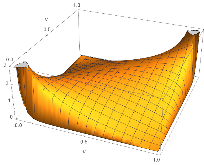
Fig. 3. Plot of for the infamous Gaussian copula. It is often not obvious to decide from the plot whether a copula has tail dependencies. In this case, Gaussian has none.

Copula Types and Generators

The most commonly used bivariate types and those implemented in ArbitrageLab are Gumbel, Frank, Clayton, Joe, N13, N14, Gaussian, and Student-t. All of those except for Gaussian and Student-t copulas fall into the category of Archimedean copulas, and Gaussian, Student-t are regarded as Elliptical copulas. Any linear combinations of those copulas with positive weights adding up to 1 will lead to mixed copulas.

Archimedean Copulas and Their Generators

(Definition of Archimedean Copula) A bivariate copula is called Archimedean if it can be represented as:
\begin{alignat*}{2}
C(u_1, u_2; \theta) = \phi^{[-1]}(\phi(u_1; \theta) + \phi(u_2; \theta))
\end{alignat*}
where is called the generator for the copula, is its pseudo-inverse, defined as
\begin{alignat*}{2}
\phi^{[-1]}(t;\theta)=
\begin{cases}
\phi^{-1}(t;\theta), \quad 0 \le t \le \phi(0; \theta) \\
0, \quad \phi(0; \theta) \le t \le \infty
\end{cases}
\end{alignat*}
As a result, one uses a generator to define an Archimedean copula. The generators’ formulae are listed below:

• Gumbel: ,
• Frank: ,
• Clayton: ,
• Joe: ,
• N13: ,
• N14: ,

Again, for applications, you do not need to remember all these unless you are coding the copulas themselves. The takeaway is that Archimedean copulas are parametric, and is uniquely determined by . Loosely speaking, is the parameter that measures how “closely” the two random variables are “related”, and its exact range and interpretation are different across different Archimedean copulas.

People study Archimedean copulas because, in general, arbitrary copulas are quite difficult to work with analytically, whereas Archimedean copulas enable further examinations by having the nice structure above. Two of the most important features of the Archimedean copula are its symmetry and scalability to multiple dimensions, although a closed-form solution may not be available in higher dimensions.

Elliptical Copulas

For the Gaussian and Student-t copula, the concepts are much easier to follow: Suppose for a correlation matrix , the multivariate Gaussian copula with parameter matrix is defined as:
\begin{alignat*}{2}
C_R(\mathbf{u}) := \Phi_R(\Phi^{-1}(u_1), \Phi^{-1}(u_2)),
\end{alignat*}
where is the joint Gaussian CDF with being its covariance matrix, is the inverse of the CDF of a standard normal. Note that using a correlation matrix instead of covariance will get identical results because copulas only care about quantiles and are invariant under linear scaling.

The Student-t copula can be defined similarly, with being the degrees of freedom:
\begin{alignat*}{2}
C_{R,\nu}(\mathbf{u}) := \Phi_{R,\nu}(\Phi_{\nu}^{-1}(u_1), \Phi_{\nu}^{-1}(u_2))
\end{alignat*}
It should also be clear that scaling elliptical copulas to multiple dimensions is also trivial, and they are also symmetric.

Mixed Copula

Archimedean copulas and elliptical copulas, though powerful by themselves to capture nonlinear relations for two random variables, may suffer from the degree to which they can be calibrated to data. While using a pure empirical copula may be subject to overfitting, a mixed copula that can calibrate the upper and lower tail dependencies usually describes the dependency structure well for its flexibility.

It is pretty intuitive to understand, for example, for a Clayton-Frank-Gumbel (CFG) mixed copula, one needs to specify the ‘s, the dependency parameter for each copula component, and their positive that sum to 1. In total there are 5 parameters for CFG (3 copula parameters and 2 weights). The weights should be understood in the sense of Markov, i.e., it describes the probability of an observation coming from a component.

For example, we present the Clayton-Frank-Gumbel mixed copula as below:
\begin{alignat*}{2}
C_{mix}(u_1, u_2; \boldsymbol{\theta}, \mathbf{w}) :=
w_C C_C(u_1, u_2; \theta_C) + w_F C_F(u_1, u_2; \theta_F) + w_G C_G(u_1, u_2; \theta_G)
\end{alignat*}

Which Copula to Choose

For practical purposes, at least for the implemented trading strategies in ArbitrageLab, it is enough to understand tail dependence for each copula and what structures are they generally modeling because sometimes the nuances only come into play for a (math) analyst.

Here are a few key results:

1. Upper tail dependence means the two random variables are likely to have extremely large values together. For instance, when working with returns series, upper tail dependence implies that the two stocks are likely to have large gains together.
2. Lower tail dependence means the two random variables are likely to have small values together. This is much stronger in general compared to upper tail dependence, because stocks are more likely to go down together than going up.
3. Frank and Gaussian copulas do not have tail dependencies at all. And Gaussian copula infamously contributed to the 2008 financial crisis by pricing CDOs exactly for this reason.
4. Frank copula has a stronger dependence in the center compared to Gaussian.
5. For Value-at-Risk calculations, Gaussian copula is overly optimistic and Gumbel is too pessimistic [Kole et al., 2007].
6. Copulas with upper tail dependence: Gumbel, Joe, N13, N14, Student-t.
7. Copulas with lower tail dependence: Clayton, N14 (weaker than upper tail), Student-t.
8. Copulas with no tail dependence: Gaussian, Frank.

Now we can look back at the mystery at the very beginning of the article on what went wrong: The bivariate Gaussian distribution assumes 1. All marginal random variables are Gaussian; 2. The copula that relates the two Gaussian marginals is also Gaussian. A Gaussian copula does not have any tail dependence. What’s worse, it requires symmetry on both upward co-moves and downward moves. Those assumptions are very rigid, and they just can’t compete with dedicated copula models for flexibility.

Open Problems

Copula is still a relatively modern concept in probability theory and finance. There are still a lot of interesting open problems to consider, and being able to solve any of these below will guarantee an edge on someone’s copula model.

1. Parametrically fit a Student-t and mixed copula.
2. Existence of statistical properties that justify two random variables to have an Archimedean copula (like one can justify a random variable is normal) [Nelsen, 2003].
3. Take advantage of copula’s ability to capture nonlinear dependencies but also adjust it for time series, so that the sequence of data coming in makes a difference.
4. Analysis of copulas when it is used on time series instead of independent draws. (For example, how different it is when working with the average on time series, compared to the average on a random variable?)
5. Adjust copulas so it can model when dependency structure changes with time.
6. All copulas mentioned, “pure” or mixed, assume symmetry. It would be nice to see an analysis of asymmetric pairs modeled by copulas.
7. The common trading logics used for copulas are still relatively primitive and can be considered a fancier version of a distance strategy and hence there is room for improvements.
8. A careful analysis done on goodness-of-fit for using copulas with tail dependencies versus those without, for various markets and various times, especially when markets are having large swings.

Check out our lecture on the topic:

References

- Liew, R.Q. and Wu, Y., 2013. Pairs trading: A copula approach. Journal of Derivatives & Hedge Funds, 19 (1), pp.12-30.
- Stander, Y., Marais, D. and Botha, I., 2013. Trading strategies with copulas. Journal of Economic and Financial Sciences, 6 (1), pp.83-107.
- Schmid, F., Schmidt, R., Blumentritt, T., Gaißer, S. and Ruppert, M., 2010. Copula-based measures of multivariate association. In Copula theory and its applications (pp. 209-236). Springer, Berlin, Heidelberg.
- Huard, D., Évin, G. and Favre, A.C., 2006. Bayesian copula selection. Computational Statistics & Data Analysis, 51 (2), pp.809-822.
- Kole, E., Koedijk, K. and Verbeek, M., 2007. Selecting copulas for risk management. Journal of Banking & Finance, 31 (8), pp.2405-2423.
- Nelsen, R.B., 2003, September. Properties and applications of copulas: A brief survey. In Proceedings of the first brazilian conference on statistical modeling in insurance and finance (pp. 10-28). University Press USP Sao Paulo.
- Cai, Z. and Wang, X., 2014. Selection of mixed copula model via penalized likelihood. Journal of the American Statistical Association, 109 (506), pp.788-801.
- Liu, B.Y., Ji, Q. and Fan, Y., 2017. A new time-varying optimal copula model identifying the dependence across markets. Quantitative Finance, 17 (3), pp.437-453.
- Demarta, S. and McNeil, A.J., 2005. The t copula and related copulas. International statistical review, 73 (1), pp.111-129.
- Nelsen, R.B., 2007. An introduction to copulas. Springer Science & Business Media.