Copula for Pairs Trading: Sampling and Fitting to Data

by Hansen Pei

Join the Reading Group and Community: Stay up to date with the latest developments in Financial Machine Learning!

LEARN MORE ABOUT PAIRS TRADING STRATEGIES WITH “THE DEFINITIVE GUIDE TO PAIRS TRADING”

This is the second article of the copula-based statistical arbitrage series. You can read the first article: Copula for Pairs Trading: A Detailed, But Practical Introduction.

Overview

Whether it is for pairs trading or risk management, two natural questions to ask before putting copula for use are: How to draw samples from a copula? How should one fit a copula to data? The necessity of fitting is quite obvious, otherwise, there is no way to calibrate our model for pairs trading or risk analysis using historical data.

For sampling, it is mostly for making a Q-Q plot against the historical data as a sanity check. Note that a copula natively cannot generate future price time series since it treats time series data as independent draws from two random variables, and thus has no information regarding the sequence, which is vital in time series analysis. One way to think about sampling from a copula trained by time series is that it gives the likelihood of where the next data point is going to be, regardless of the input sequence.

The former question about sampling has an analytical answer for all the bivariate copulas we care about (Gumbel, Clayton, Frank, Joe, N13, N14, Gaussian, Student-t, and any finite mixture of those components). As with pretty much all analytical approaches in applications, it requires a bit of mathematical elbow grease to wrap the head around a few concepts. But once employed, it is pretty fast and reliable.

The latter question about fitting to data is still somewhat open, and the methods are statistical. Therefore those are relatively easy to understand, but they might suffer from performance issues and may require active tuning of hyperparameters.

Throughout this post, we will discuss:

The method employed in sampling from a copula.
Fitting a “pure” copula to data.
Fitting a mixed copula to data using an EM algorithm.

We limit our discussion to bivariate cases unless otherwise specified. You can also refer to my previous article Copula for Pairs Trading: A Detailed, But Practical Introduction to brush up on the basics.

Another note is that all the algorithms mentioned in this article will be incorporated in the copula trading module from ArbitrageLab since version 0.3.0 so that you do not need to code them by yourself, and this article is meant to be a technical discussion for interested readers who want to know how things are implemented, where the bottlenecks are in performance, and what can and cannot be achieved intrinsically based on our current understanding of copula.

Sampling

Suppose you have a joint cumulative density function $H(x_1, x_2) = \mathbb{P}(X_1 \le x_1, X_2 \le x_2)$ and you want to sample a few points from it. Mathematically it is pretty straightforward:

Draw a number $p$ uniformly in $[0,1]$ as the probability.
Find the level curve $\Gamma = \{ (x_1, x_2) | H(x_1, x_2) = p \}$ , and draw a point uniformly from this curve via arc-length parameterization.

Done! Can we apply this to copulas? Theoretically not really, practically a hard no. Finding the level curve is in general a bad idea from a computational point of view. There exist other algorithms that perform better than the above such as Metropolis-Hastings. However, all the copulas we care about have some nice structures, and we are gonna take advantage of them.

“Pure” Copula

Note that “pure” copula is in no way a formal name. I call Archimedean and elliptical copulas together as “pure” to distinguish them from mixed copulas (in the Markovian sense, we will address it later) of Archimedean and elliptical components.

For Archimedean copulas, the general methodology for sampling or simulation comes from [Nelsen, 2007]:

Generate two uniform in $[0,1]$ i.i.d. ‘s $(v1,v2)$ .
Calculate $w = K_c^{-1}(v_2)$ , $K_c(t) = t - \frac{\phi(t)}{\phi'(t)}$ .
Calculate $u_1 = \phi^{-1}[v_1 \phi(w)]$ and $u_2 = \phi^{-1}[(1-v_1) \phi(w)]$ .
Return $(u_1, u_2)$ .

For the Frank and Clayton copula, the above method can greatly be simplified due to having closed-form solutions for step 2. Otherwise, one will have to use appropriate numerical methods to find w. Interested readers can check Procedure to Generate Uniform Random Variates from Each Copula for some of the simplified forms.

For Gaussian and Student-t copulas, one can follow the procedures below:

Generate a pair $(v_1, v_2)$ using a bivariate Gaussian/Student-t distribution with desired correlation (and degrees of freedom).
Transform those into quantiles using CDF from standard Gaussian or Student-t distribution (with desired degrees of freedom). i.e., $u_1 = \Phi(v_1)$ , $u_2 = \Phi(v_2)$ .
Return $(u_1, u_2)$

Mixed Copula

A mixed copula has two sets of parameters: parameters corresponding to the dependency structure for each component copula (let’s call them copula parameters for reference) and positive weights that sum to 1. For example, we present the Clayton-Frank-Gumbel mixed copula as below:

$C_{mix}(u_1, u_2; \boldsymbol{\theta}, \mathbf{w}) := w_C C_C(u_1, u_2; \theta_C) + w_F C_F(u_1, u_2; \theta_F) + w_G C_G(u_1, u_2; \theta_G)$

The weights should be interpreted in the Markovian sense, i.e., the probability of an observation coming from a component. (Do not confuse them with the BB families where the mixture happens at the generator level.) Then sampling from a mixed copula becomes easy: for each new sample, just choose a component copula with associated probability, and generate a pair from that copula.

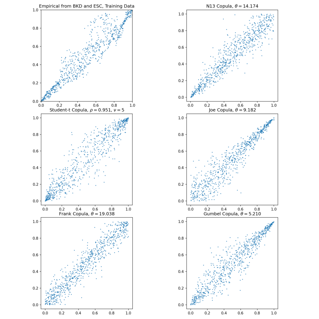
Empirical copula and sampled N13, Student-t, Joe, Frank, and Gumbel copulas.

Fitting to Data

This is an active research field. Here we are just introducing some commonly used methods. Note that every fitting method should come with a way for evaluation. For the same dataset, one can use the classic sum of log-likelihood, or various information criteria like AIC, SIC, and HQIC by also taking account of the number of parameters and sample size. For evaluations across datasets, there currently are no widely accepted methods.

Now, we face two issues for fitting:

How to translate marginal data into quantiles?
How to fit a copula with quantiles?

Maximum Likelihood and ECDF

All copulas we have mentioned so far are parametric, i.e., they can be defined uniquely by parameter(s). Hence it is possible to wrap an optimizer over the model and set the sum of log-likelihood generated from copula density $c(u_1, u_2)$ as the objective function to maximize. However this is slow, and with $4$ or $5$ parameters to fit even for a bivariate “pure” copula with arbitrary marginal distributions it may not be ideal. Hence we usually do not go for this approach, and the empirical CDFs (ECDFs) are generally used instead.

Note that using ECDF will require the marginal random variable to be approximately stationary, otherwise they may go out of bound of a training set infinitely often. This can happen when one fits copula to two stocks prices time series when at least one of them has a positive drift, then the marginal quantile will almost surely be one after a certain point.

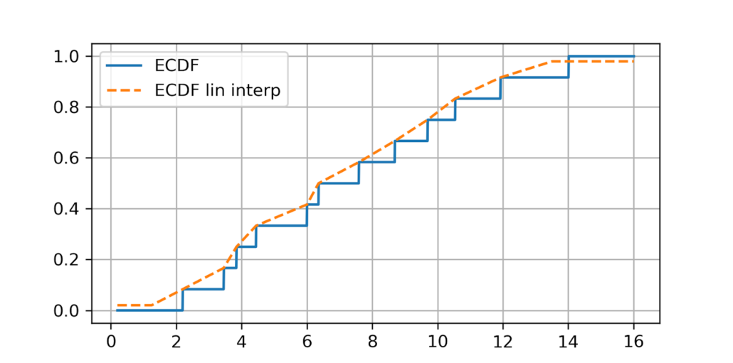
Also, the ECDF function provided by a statsmodels library is a step function. And it thus does not work well where the density of data is thin. A nice adaptation is to use linear interpolations between the steps. Moreover, it makes computational sense to wrap the ECDF’s value within $[\varepsilon, 1-\varepsilon]$ to avoid edge results in 0 or 1, which may lead to infinite values in copula density and screw up the fitting process. We provide the modified ECDF in the copula module as well, and by default, all trading modules are built based on it. See the picture below for comparison:

ECDF vs. ECDF with linear interpolation. The max on the training data 14, the min is 2.2. We made the $\varepsilon$ for upper and lower bound much larger on our ECDF for visual effect.

Pseudo-Maximum likelihood

We follow a two-step pseudo-MLE approach as below:

Use Empirical CDF (ECDF) to map each marginal data to its quantile.
Calculate Kendall’s $\hat\tau$ for the quantile data, and use Kendall’s $\hat\tau$ to calculate $\hat\theta$ .

For elliptical copulas, $\theta$ estimated here is their $\rho$ , the correlation parameter.

For Archimedean copulas, $\tau$ and $\theta$ are implicitly related via

$\tau(\theta) = 1 + 4 \int_0^1 \frac{\phi(t;\theta)}{\phi'(t;\theta)} dt$

Then one inversely solves $\hat\theta(\hat\tau)$ . For some copulas, the inversion has a closed-form solution. For others, one has to use numerical methods.

For elliptical copulas, we calculate Kendall’s $\hat{\tau}$ and then find $\hat{\rho}$ via

$\hat{\rho} = \sin \left( \frac{\hat{\tau} \pi}{2} \right)$

for the covariance matrix $\mathbf{\sigma}_{2 \times 2}$ (though technically speaking, for bivariate copulas, only correlation $\rho$ is needed, and thus it is uniquely determined) from the quantile data, then use $\mathbf{\sigma}_{2 \times 2}$ for a Gaussian or Student-t copula. Fitting by Spearman’s $\rho$ is the variance-covariance matrix from data for elliptic copulas is also practised by some. But Spearman’s $\rho$ is, in general, less stable than Kendall’s $\tau$ (though with faster calculation speed). And using variance-covariance implicitly assumes a multivariate Gaussian model, and it is sensitive to outliers.

A Note about Student-t Copula

Theoretically speaking, for Student-t copula, determining $\nu$ (degrees of freedom) analytically from an arbitrary time series is still an open problem. Therefore we opted to use a maximum likelihood fit for $\nu$ for the family of Student-t copulas initiated by $\mathbf{\sigma}_{2 \times 2}$ . This calculation is relatively slow.

EM Two-Step Method for Mixed Copula

Specific Problems with Maximum Likelihood

Archimedean copulas and elliptical copulas, though powerful by themselves to capture nonlinear relations for two random variables, may suffer from the degree to which they can be calibrated to data, especially near the tails. While using a pure empirical copula may be subject to overfitting, a mixed copula that can calibrate the upper and lower tail dependence usually describes the dependency structure well for its flexibility.

But this flexibility comes at a price: fitting it to data is far from trivial. Although one can, in principle, wrap an optimization function for finding the individual weights and copula parameters using max likelihood, realistically this is a bad practice for the following reasons:

The outcome is highly unstable and is heavily subject to the choice of the maximization algorithm.
A maximization algorithm fitting 5 parameters for a Clayton-Frank-Gumbel (CFG) or 6 parameters for Clayton-Student-Gumbel (CTG) usually tends to settle to a bad result that does not yield a comparable advantage to even its component copula. For example, sometimes the fit score for CTG is worse than a direct pseudo-max likelihood fit for Student-t copula.
Sometimes there is no result for the fit since the algorithm does not converge.
Some maximization algorithms use a Jacobian or Hessian matrix, and for some copulas, the derivative computation does not numerically stay stable.
Often the weight of a copula component is way too small to be reasonable. For example, when an algorithm says there is 0.1% Gumbel copula weight in a dataset of 1000 observations, then there is on average 1 observation that comes from that Gumbel copula. It is just bad modeling in every sense.

The EM Algorithm

Instead, we adopt a two-step expectation-maximization (EM) algorithm for fitting mixed copulas, adapted from [Cai, Wang 2014]. This algorithm addresses all the above disadvantages of a generic maximization optimizer. The only obvious downside is that the CTG copula may take a while to converge to a solution for certain data sets.

Suppose we are working on a three-component mixed copula of bivariate Archimedeans and ellipticals. We aim to maximize the objective function for copula parameters $\boldsymbol{\theta}$ and weights $\mathbf{w}$ .

$Q(\boldsymbol{\theta}, \mathbf{w}) = \sum_{t=1}^T \log \left[ \sum_{k=1}^3 w_k c_k(u_{1,t}, u_{2,t}; \theta_k) \right] - T \sum_{k=1}^3 p_{\gamma, a}(w_k) + \delta \left( \sum_{k=1}^s w_k - 1 \right),$

where $T$ is the length of the training set or the size of the observations; $k$ is the dummy variable for each copula component; $p_{\gamma, a}(\cdot)$ is the smoothly clipped absolute deviation (SCAD) penalty term with tuning parameters $\gamma$ and $a$ and it is the term that drives small copula components to $0$ ; and last but not least $\delta$ the Lagrange multiplier term that will be used for the E-step is:

$\delta = T p'_{\gamma, a}(w_k) - \sum_{t=1}^T \frac{c_k(u_{1,t}, u_{2,t}; \theta_k)} {\sum_{j=1}^3 w_{j} c_{j}(u_{1,t}, u_{2,t}; \theta_{j})}$

E-step

Iteratively calculate the following using the old $\boldsymbol{\theta}$ and $\mathbf{w}$ until it converges:

$w_k^{new} = \left[ w_k p'_{\gamma, a}(w_k) - \frac{1}{T} \sum_{t=1}^T \frac{c_k(u_{1,t}, u_{2,t}; \theta_k)} {\sum_{j=1}^3 w_{j} c_{j}(u_{1,t}, u_{2,t}; \theta_{j})} \right] \times \left[ \sum_{j=1}^3 w_{j} p'_{\gamma, a}(w_{j}) \right]^{-1}$

M-step

Use the updated weights to find new $\boldsymbol{\theta}$ , such that $Q$ is maximized. One can use truncated Newton or Newton-Raphson for this step. This step, though still a wrapper around some optimization function, is much better than estimating the weights and copula parameters altogether.

We then iterate the two steps until it converges. It is tested that the EM algorithm is oracle and sparse. Loosely speaking, the former means it has good asymptotic properties, and the latter says it will trim small weights off.

Possible Issues Discussion

The EM algorithm is still not mathematically perfect, and has the following issues:

It is slow for some data sets. Specifically, the CTG is slow due to the bottleneck from Student-t copula.
If the copulas mixture has similar components, for instance, Gaussian and Frank, then it cannot pick the correct component weights well. Luckily for fitting data, usually the differences are minimal.
The SCAD parameters $\gamma$ and $a$ may require some tuning, depending on the data set it fits. Some literature suggested using cross-validation to find a good pair of values. We did not implement this in the ArbitrageLab because it takes quite long for the calculation to a point it becomes unrealistic to run it.
Sometimes the algorithm taken from scipy.optimization package throws warnings because the optimization algorithm underneath does not strictly follow the prescribed bounds. Usually, this is not an issue that will compromise the result, and some minor tunings on SCAD parameters can solve this issue.
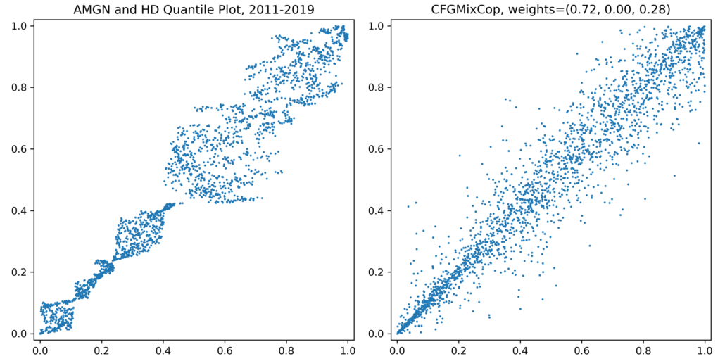
Sometimes the pattern in the data cannot be explained well by any of our copulas, even if they are initially selected by Kendall’s tau or Euclidean distance, very likely to co-move together and thus have the potential for pairs trading. See below for an example of price data. Changing to returns data usually will be much better for fitting, but the data will have much more noise, and trading algorithms should be designed specifically with this into consideration.

References

- Schmid, F., Schmidt, R., Blumentritt, T., Gaißer, S. and Ruppert, M., 2010. Copula-based measures of multivariate association. In Copula theory and its applications (pp. 209-236). Springer, Berlin, Heidelberg.
- Huard, D., Évin, G. and Favre, A.C., 2006. Bayesian copula selection. Computational Statistics & Data Analysis, 51(2), pp.809-822.
- Nelsen, R.B., 2003, September. Properties and applications of copulas: A brief survey. In Proceedings of the first brazilian conference on statistical modeling in insurance and finance (pp. 10-28). University Press USP Sao Paulo.
- Cai, Z. and Wang, X., 2014. Selection of mixed copula model via penalized likelihood. Journal of the American Statistical Association, 109(506), pp.788-801.
- Nelsen, R.B., 2007. An introduction to copulas. Springer Science & Business Media.