The Correct Vectorized Backtest Methodology for Pairs Trading

by Hansen Pei

Join the Reading Group and Community: Stay up to date with the latest developments in Financial Machine Learning!

LEARN MORE ABOUT PAIRS TRADING STRATEGIES WITH “THE DEFINITIVE GUIDE TO PAIRS TRADING”

Vectorized Backtesting and Pairs Trading

Whilst backtesting architectures is a topic on its own, this article dives into how to correctly backtest a pairs trading investment strategy using a vectorized (quick methodology) rather than the more robust event-driven architecture. This is a technique that is very common amongst analysts and is rather straightforward for long-only portfolios, however, when you start to construct long-short portfolios based on statistical arbitrage, strange little nuances start to pop up.

Please note that we are strongly advocating against research through backtesting and encourage you to turn to tools such as feature importance, to guide the process. A backtest is the very last sanity check and one needs to be very careful of generating false investment strategies.

Let’s dive in!

What is an Equity Curve

Forming an equity curve is usually regarded as a sanity check on strategies to have a glance over their performance. It can be thought of as a quick backtest, usually composed of a few lines of code, focused on the strategy itself without worrying too much about VaR, transaction costs, market impact, slippage, frictions, etc., which can be handled by various full-on backtest platforms.

“Oh, it is just calculating the excess returns over some positions. What is the big deal?”

Ideally, it is simple. However, it is like one of those “trivial and left as an exercise to the reader” marks in an abstract algebra textbook. Maybe it is, for this reason, there is little discussion on it when it becomes non-trivial.

Serge Lang, Algebra.

Here is one interesting problem to ponder: How to calculate returns of an arbitrage opportunity? Well, if you can make chunks of gold out of thin air, infinitely, with no cost and no risk, this kind of arbitrage has infinite returns. But, say that you are running a statistical arbitrage: pairs trade over two stocks X and Y and you find a lucrative algorithm adapted from some literature. The algorithm suggests that you should long the spread of X and Y (i.e., long X and short Y with correct hedge ratio) when the spread is $0, and exit when the spread is $1. You followed the algorithm, and to make this discussion simple, say you longed X and shorted Y by exactly 1 unit. In the end, you made 1 dollar, now the question is, what is the return? (Hint: infinity is not a correct answer.)

Through this article I aim to cover the following topics:

Calculate the equity curve for a single stock.
Calculate the equity curve for two stocks, including long-only and long-short.
Interpretation of returns for a dollar-neutral strategy.
Common fallacies in the equity curve calculation.

Non-Trivial Issues

The major issue comes in if the assets that we calculate the equity curve upon, are not all the same. It is not difficult to calculate equity curves for a single stock, however, things change when the underlying becomes a portfolio, especially when long and short positions for each component are allowed. For pairs trading, a long-short portfolio (spread) is in a sense self-financing: You can (depending on your broker) cover the long position cost (at least partially) from the short position. And when this happens, the usual definition of returns stops working since the cost of investment becomes unclear, and it may appear one just made gold out of thin air and returns become infinity.

Another issue is about calculating the value of a portfolio. Just like the value of common stock, one wishes to see how it evolves, and visually see where to take long and short positions to capture opportunities. We will demonstrate later that this may not work for some types of strategies.

Valid Methods for Forming an Equity Curve

Here we provide a few frameworks for calculating equity curves with valid logic. A very important note here is that they work with different objects. We will discuss the common mistakes that arise from misuse.

Returns: Single Stock

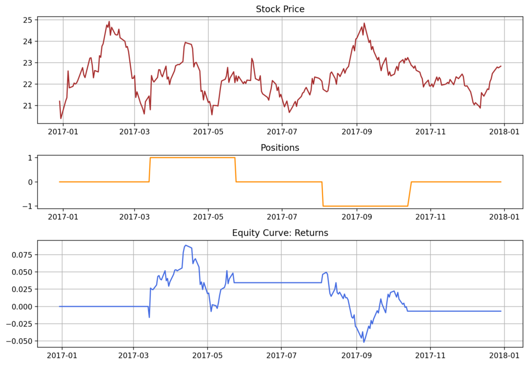
This is rather straightforward, but note that stock prices cannot go negative. In this case, we are essentially capturing the daily returns, and thus forming an equity curve on returns.

Get the stock price $S$ .
Get stock’s daily returns series.
$r(t) = \frac{S(t)}{S(t-1)} -1$
Get the positions $P(t)$ from a strategy, for the position held on that day (Be very careful not to introduce look-ahead bias in this step!).
Calculate the daily returns $r_s(t)$ from our strategy. It is the pointwise multiplication
$r_s(t) = r(t)P(t), \ \text{for each} \ t$
Then we use daily returns $r_s(t)$ to cumulatively reconstruct our portfolio’s equity curve on returns:
$\mathcal{E}(t) = \left( \prod_{\tau=0}^t [r_s(\tau) + 1] \right) - 1$

Note: We assume the positions series $P(t)$ is a time series of (bounded) real numbers, indicating how many units of the portfolio to hold at time $t$ , suggested by some strategy. For some strategies, it only takes values from $\{0, 1, -1\}$ , representing no position, 100% long and 100% short respectively.

# 1. Portfolio time series
prices = testing_data['GDX']

# 2. Portfolio's returns
rts = prices.pct_change()

# 3. Suggested positions by some strategy
# I am just making the positions up for ease of demonstration.
position_data = [0]*50 + [1]*50 + [0]*50 + [-1]*50 + [0]*53
positions = pd.Series(data=position_data, index=prices.index)

# 4. Returns from our strategy
rts_strat = rts * positions

# 5. (Normalized) P&L
equity_normalized = (1 + rts_strat).cumprod() - 1

Forming a Portfolio from a Pair of Stocks

To keep things simple for now, suppose we have 2 stocks in the portfolio, with non-negative value time series $S_A$ , $S_B$ . The portfolio’s value time series is defined as

$\Pi(t) = w_A(t) S_A(t) + w_A(t) S_B(t),$

where $w_A$ and $w_B$ are units held for $S_A$ and $S_B$ , and they can be any real number: They do not necessarily sum to 1 and they do not need to be positive.

For a long-only portfolio, we assume the units held are non-negative. Moreover, it is common to normalize by letting the units be a partition of $[0,1]$ if they are constants, and they effectively become weights, i.e.,

$w_A + w_B = 1; \quad w_A, w_B \ge 0.$

For a long-short portfolio, hedge ratio $h(t)$ is generally used for the number of units held. Here we use it as:

$w_A = 1, \quad w_B(t) = -h(t).$

Generally, $h$ should be a function of time, but occasionally it is constant during the trading period (for instance, one calculates it from OLS on training data for benchmarking). The long-short portfolio formed from the hedge ratio thus has a value time series as:

$\Pi(t) = S_A(t) - h(t) S_B(t),$

Returns: Long-Only Portfolios

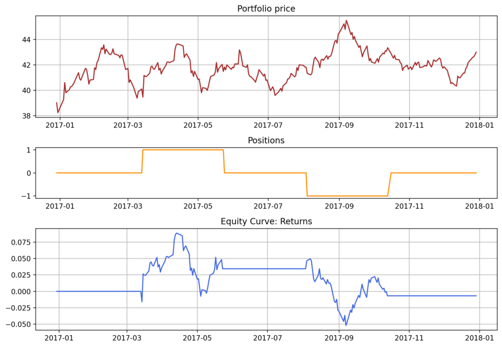
Suppose we have positive units held $w_A(t), w_B(t)$ on two strictly positive value time series (stocks, funds, etc.). The method applied to a single stock still works.

Construct the portfolio (price series) $\Pi$ .
$\Pi(t) = w_A(t) S_A(t) + w_B(t) S_B(t)$
Get the portfolio’s daily returns series.
$r(t) = \frac{\Pi(t)}{\Pi(t-1)} - 1$
Get the positions $P(t)$ from a strategy, held on that day.
Calculate the daily returns $r_s(t)$ from our strategy. It is the pointwise multiplication
$r_s(t) = r(t)P(t), \ \text{for each} \ t$
Then we use daily returns $r_s(t)$ to reconstruct our portfolio’s equity curve on returns:
$\mathcal{E}(t) = \left( \prod_{\tau=0}^t [r_s(\tau) + 1] \right) - 1$

# 1. Portfolio time series
# Weights are arbitrarily chosen as a partition of [0, 1] for demonstration
w1 = 0.8  # Positive weight
w2 = 0.2  # Positive weight
portfolio = w1 * testing_data['GDX'] + w2 * testing_data['GLD']

# 2. Portfolio's returns
rts = portfolio.pct_change()

# 3. Suggested positions by some strategy
# I am just making the positions up for ease of demonstration.
position_data = [0]*50 + [1]*50 + [0]*50 + [-1]*50 + [0]*53
positions = pd.Series(data=position_data, index=portfolio.index)

# 4. Returns from our strategy
rts_strat = rts * positions

# 5. (Normalized) P&L
equity_normalized = (1 + rts_strat).cumprod() - 1

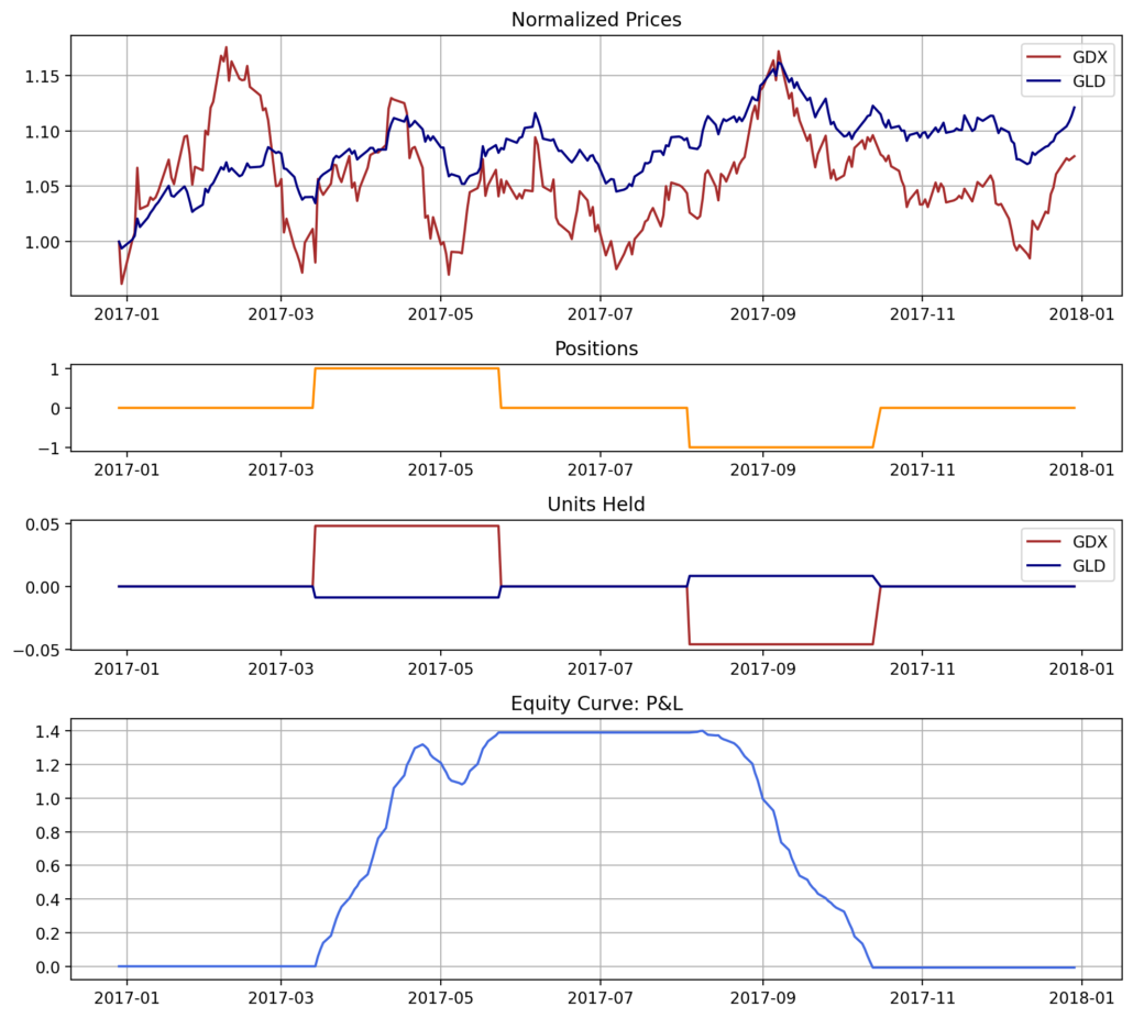
Daily Profit and Loss (P&L): Long-Short Portfolios and Others

Daily profit and loss (P&L) is the most general approach and it should work for all portfolios. Specifically for a long-short pair’s trading portfolio, where the portfolio value time series can be positive, negative, or switching around 0, this method will provide the correct information. We provide the calculation procedure for a long-short stocks pair portfolio:

Construct the portfolio (price series) $\Pi$ with some hedge ratio.
$\Pi(t) = S_A(t) - h(t) S_B(t)$
Get the portfolio’s daily revenue (price difference, daily P&L for one unit) series.
$R(t) = \Pi(t) - \Pi(t-1)$
Get the positions $P(t)$ from a strategy.
Calculate the daily returns $Rs(t)$ from our strategy. It is the pointwise multiplication
$R_s(t) = R(t)P(t), \ \text{for each} \ t$
Then we use daily P&L $R_s(t)$ to reconstruct our portfolio’s equity curve on P&L:
$\mathcal{E}(t) = \sum_{\tau=0}^t R_s(\tau)$

This can be interpreted as the (cumulative) P&L for holding a single unit of the portfolio, with given positions suggested by the strategy.

h_ols = 1.4  # Hedge ratio suggested by OLS on training data
# 1. Portfolio time series
portfolio = testing_data['GDX'] - h_ols * testing_data['GLD']

# 2. Portfolio's daily P&L for holding 1 unit
pnl = portfolio.diff()

# 3. Suggested positions by some strategy
# I am just making the positions up for ease of demonstration.
position_data = [0]*50 + [1]*50 + [0]*50 + [-1]*50 + [0]*53
positions = pd.Series(data=position_data, index=portfolio.index)

# 4. Daily P&L from our strategy
pnl_strat = pnl * positions

# 5. Equity curve
equity_pnl = (pnl_strat).cumsum()

Returns-ish: Dollar-Neutral

As mentioned in Gatev et al., 2006 for its proposed distance-based strategy, the trader takes 1 dollar short in the higher-priced stock and 1 dollar long for the lower-priced stock. In this case, there is no such thing as a standalone portfolio value time series evolving by itself.

We can still calculate the daily P&L, and then form an equity curve. Note that the P&L is computed over long-short positions for 1 dollar, it can somewhat be interpreted as “returns”. However, we still need to keep in mind that this is fundamentally different from the returns for the case when someone just bought 1 dollar worth of some stocks because this 1 dollar is not the actual principal, it is just an arbitrary bound.

# Use the MPI module in the copula approach library for calculating dollar neutral units
CS = csmpi.CopulaStrategyMPI()

# I am just making the positions up for ease of demonstration.
position_data = [0]*50 + [1]*50 + [0]*50 + [-1]*50 + [0]*53
positions = pd.Series(data=position_data, index=portfolio.index)

# The method used below splits 1 dollar into long and short positions equally, hence adjust multiplier = 2
units = CS.positions_to_units_dollar_neutral(prices_df=testing_data, positions=positions, multiplier=2)

# Get the portfolio's daily P&L, which is the number of units held multiplying with prices
portfolio_pnl = units['GDX'] * testing_data['GDX'] + units['GLD'] * testing_data['GLD']

# Cumulatively sum the daily P&L for the equity curve
equity = portfolio_pnl.cumsum()

Common Mistakes

Linearly Combining Returns

When calculating the portfolio prices by itself, the returns $r(t)$ is

$r(t) = \frac{ \Pi(t) } { \Pi(t-1) } - 1$

$r(t) = \frac{w_A(t) S_A(t) + w_B(t) S_B(t)}{w_A(t-1) S_A(t-1) + w_B(t-1) S_B(t-1)} -1 \neq w_A(t) r_A(t) + w_B(t) r_B(t)$

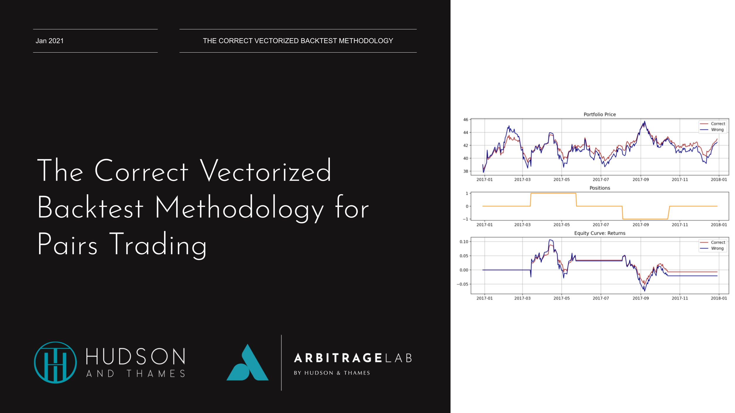
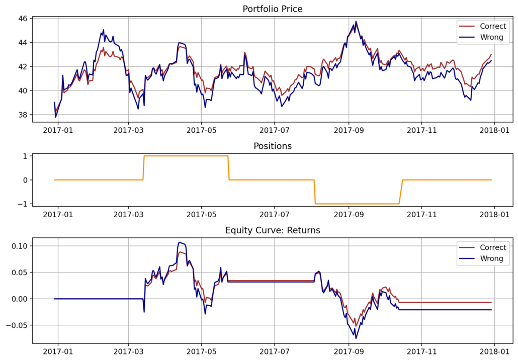
In plain English, it means you cannot linearly combine the returns from each component to calculate returns for the portfolio. If the weights are chosen well, the wrong equity curve will be around the correct equity curve so it is not completely the end of the world. The correct way to calculate $r(t)$ is the left side of the above equation: by forming the portfolio’s value series from each component, then calculate the excess returns. The weights need to be positive as well.

Using the Long-Only Method on Other Portfolios

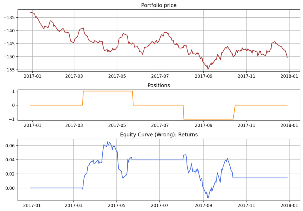
The method for calculating long-only portfolios should be applied to long-only portfolios. If used on a long-short portfolio, or where a component’s value time series does not stay positive, it will break down.

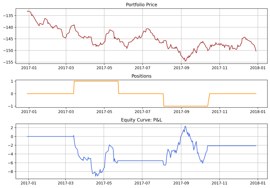
See below for a wrong implementation on a negative time series using the method that was intended for long-only portfolios. We end up getting the opposite of what we are looking for.

The logic breaks down when calculating returns of the portfolio, due to $\Pi(t)$ not being strictly positive, and this invalidates the calculation of the return.

References

Gatev, E., Goetzmann, W.N. and Rouwenhorst, K.G., 2006. Pairs Trading: Performance of a Relative-Value Arbitrage Rule. The Review of Financial Studies, 19 (3).