There are 6 properties that empirical correlation matrices exhibit that no synthetic generation method has been able to replicate, until now.

Enabling researchers to backtest strategies on an abundance of data would make our algorithms and strategies more robust, accurate, and efficient. Since historical data can be biased and does not have enough high-stress events to test multiple scenarios, generating synthetic data is a practical way to overcome this problem. However, generating data that is realistic is not an easy task. Realistic data, especially financial data, has many special characteristics that if not taken into account, would make any backtested strategy useless.

Historical financial data has many limitations. First, they are prohibitively expensive for many users. Acquiring historical, reliable, bias-free, stock returns data can cost thousands of dollars without taking into account infrastructure costs.

Next, financial data contains sensitive and personally identifiable attributes of customers. Sharing this data, even between the same organization, can be difficult and restrictive.

Furthermore, they are biased due to historical events happening in only one way. They do not explore different possibilities and different scenarios. Historical data is only available for one of the many branches of history.

Additionally, there is a lack of important events. For example, flash crashes, world-wide economic crises, global pandemics, etc. Without this data, it is difficult to assess if an algorithm will fare well for any event. There is no easy way to test for different and realistic what-if scenarios. Having an abundance of realistic financial data also can help fight against the dangers of overfitting.

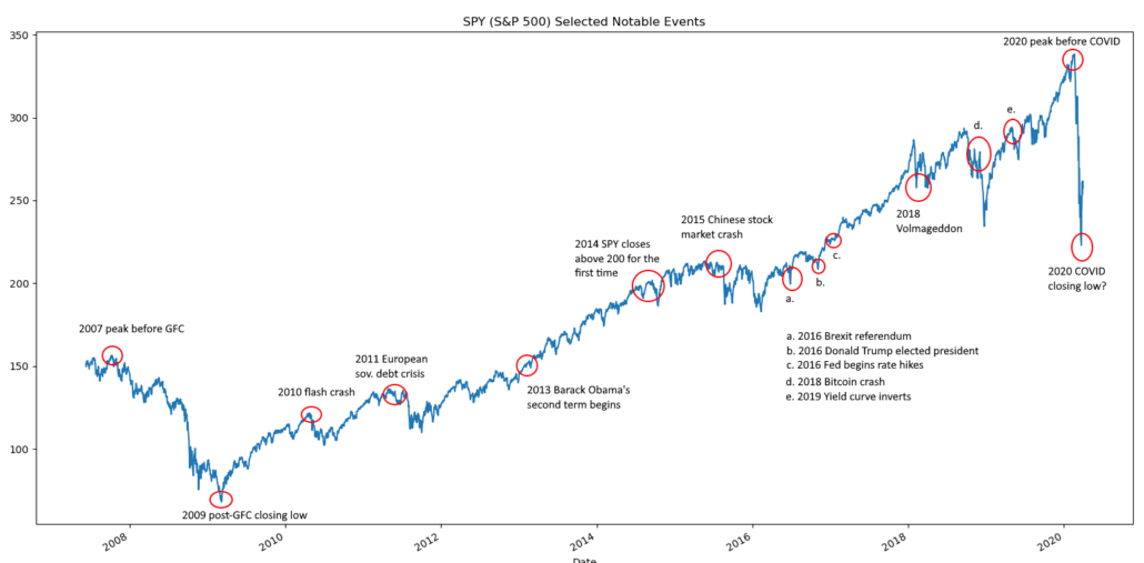
Figure 1. In 13 years of data (about 3k days), we show just a few notable events (15). Not enough for reliable and robust tests.

Examples of financial data that can be generated include stock prices, stock returns, correlation matrices, retail banking data, and all kinds of market microstructure data. We are trying to close that gap and generate realistic financial data.

Correlation Matrices

Financial correlation matrices are constructed by using the correlation of stock returns over a specified time frame. Usually, the Pearson’s correlation coefficient is used to measure their linear correlation and codependence. There are other methods to measure codependence not covered here. For more information, check out our documentation and implementations of Codependence.

Correlation matrices are useful for risk management, asset allocation, hedging instrument selection, pricing models, etc. According to (Laloux et al, 200):

“The probability of large losses for a certain portfolio or option book is dominated by correlated moves of its different constituents — for example, a position which is simultaneously long in stocks and short in bonds will be risky because stocks and bonds usually move in opposite directions in crisis periods.”

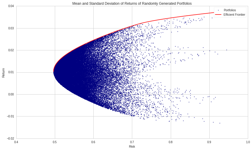
For example, in mean-variance optimization of portfolios, risk and return are measured by the variance and mean of the portfolio returns. One way to calculate the variance of a portfolio is by using the covariance matrix of its returns. Usually, this covariance matrix is estimated from historical data, which makes it subject to estimation errors.

Figure 2. Efficiency frontier of several hypothetical portfolios. The objective is to optimize a portfolio’s return relative to risk (risk is assessed, in part, by the covariance matrix of returns) (Abasi, Margenot and Granizo-Mackenzie, 2020)

There have been many attempts to generate synthetic correlation matrices, but according to (Hüttner, Mai and Mineo, 2018)

“To the best of our knowledge, there is no algorithm available for the generation of reasonably random [financial] correlation matrices with the Perron-Frobenius property.”

“Concerning the generation of [financial] correlation matrices whose MSTs [Minimum Spanning Trees] exhibit the scale-free property, to the best of our knowledge there is no algorithm available, and due to the generating mechanism of the MST we  expect  the  task  of  finding  such  correlation matrices to be highly complex”

Empirical financial correlation matrices exhibit certain ‘stylized facts’ that researchers have found (Marti 2020a):

1. Distribution of pairwise correlations is significantly shifted to the positive
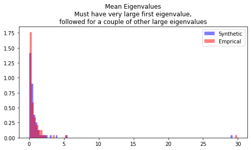
2. Eigenvalues follow the Marchenko-Pastur distribution, but for a very large first eigenvalue (the market).
3. Eigenvalues follow the Marchenko-Pastur distribution, but for a couple of other large eigenvalues (industries)
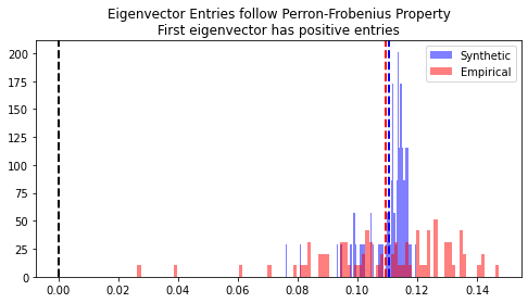
4. Perron-Frobenius property (first eigenvector has positive entries).
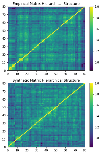
5. Hierarchical structure of correlations.
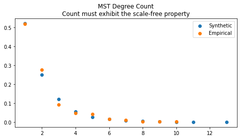
6. Scale-free property of the corresponding Minimum Spanning Tree (MST).

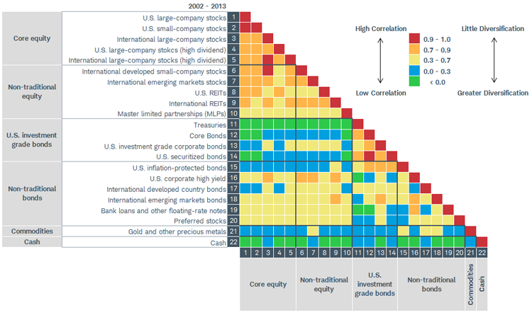
Figure 3. Sample Financial Correlation Matrix (Courtesy of Schwab Intelligent Portfolios™ Asset Allocation White Paper).

CorrGAN

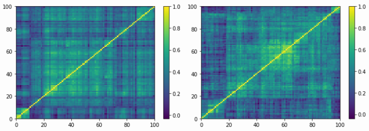
Previous methods found (Marti 2020a) for generating realistic correlation matrices were lacking. These methods are not able to reproduce all of these “stylized facts”. Dr. Marti’s CorrGAN addressed this problem by using a Generative Adversarial Network (GAN) (Marti 2020a) .

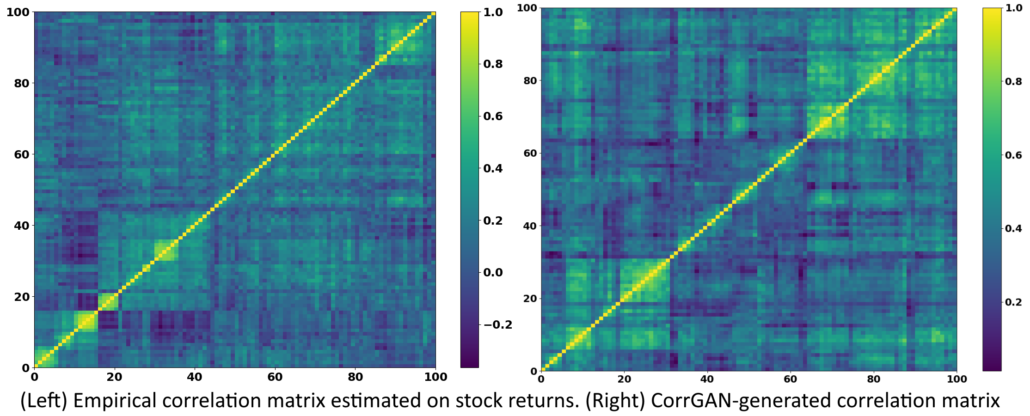
Figure 4. (Left) Empirical correlation matrix estimated on stock returns; (Right) GAN-generated correlation matrix (Marti 2020b).

GANs are a type of neural network designed by Ian Goodfellow. It is an unsupervised learning method where two neural networks ‘compete’ with each other. One network tries to fool the other by generating data that the other network is unable to classify as real or fake.

GANs are used to discover and learn the irregularities and patterns in data. This enables them to generate realistic samples drawn from the original training data. For more information and the theory behind GANs, check out the research publication by Goodfellow et al., 2014, Generative Adversarial Nets.

Recent advancements in GANs have been able to generate faces of people that never existed, but they can fool most humans on recognizing if they are fake or not.

Figure 5. Which one is real? (Courtesy of whichfaceisreal)

CorrGAN was trained on approximately 10,000 empirical correlation matrices estimated on S&P 500 returns sorted by a permutation induced by a hierarchical clustering algorithm. The result was CorrGAN! Dr. Marti was able to contrast and compare the stylized facts of the empirical and generated matrices. He found that CorrGAN is able to recover these stylized facts and produce realistic results.

Empirical and CorrGAN comparison

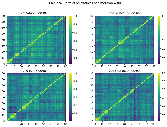
Now we are going to show how CorrGAN compares to empirical matrices. Both have a dimension of 80. The empirical matrices are from a random sample

import os
import numpy as np
import pandas as pd
import random
import matplotlib.pyplot as plt
from scipy.cluster import hierarchy
import networkx as nx
import yfinance as yf
from mlfinlab.data_generation.corrgan import sample_from_corrgan
from mlfinlab.data_generation.data_verification import plot_stylized_facts
import warnings
from IPython.display import Image
warnings.filterwarnings('ignore')

random.seed(2814)
np.random.seed(2814)

# Adapted from: https://marti.ai/ml/2019/10/13/tf-dcgan-financial-correlation-matrices.html

dimensions = 80

# Download stock returns and compute correlations.
SP_ASSETS_80 = ['FIS', 'JCI',... , 'SBAC', 'SPG']
prices = yf.download(tickers=" ".join(SP_ASSETS_80), start="2014-12-01", end="2015-09-28")['Close']
prices = prices.pct_change()
rolling_corr = prices.rolling(252, min_periods=252//2).corr().replace([np.inf, -np.inf], np.nan).dropna()
tri_rows, tri_cols = np.triu_indices(dimensions, k=1)

# Plot a few correlation matrices.
plt.figure(figsize=(12, 8))
plt.suptitle("Empirical Correlation Matrices of dimension = {}".format(dimensions))
i = 0
for date in random.sample(rolling_corr.groupby(level=0).indices.keys(), 4):
    corr_mat = rolling_corr.loc[date].values
    
    # Arrange with hierarchical clustering by maximizing the sum of the
    # similarities between adjacent leaves.
    dist = 1 - corr_mat
    linkage_mat = hierarchy.linkage(dist[tri_rows, tri_cols], method="ward")
    optimal_leaves = hierarchy.optimal_leaf_ordering(linkage_mat, dist[tri_rows, tri_cols])
    optimal_ordering = hierarchy.leaves_list(optimal_leaves)
    ordered_corr = corr_mat[optimal_ordering, :][:, optimal_ordering]
    
    # Plot it.
    plt.subplot(2, 2, i + 1)
    plt.pcolormesh(ordered_corr, cmap='viridis')
    plt.colorbar()
    plt.title(date)
    i += 1
plt.show()

Here we show a sample of the type of empirical correlation matrices CorrGAN was trained on.

Figure 6. Empirical correlation matrices comparison.

CorrGAN in mlfinlab

# Sample from CorrGAN.
corrgan_mats = sample_from_corrgan(model_loc="{}/mlfinlab/corrgan_models".format(os.getcwd()), dim=dimensions, n_samples=len(rolling_corr.index.get_level_values(0).unique()))

# Plot a few samples.
plt.figure(figsize=(12, 8))
plt.suptitle("Generated Correlation Matrices of dimension = {}".format(dimensions))
for i in range(4):
    plt.subplot(2, 2, i + 1)
    plt.pcolormesh(corrgan_mats[i], cmap='viridis')
    plt.colorbar()
plt.show()

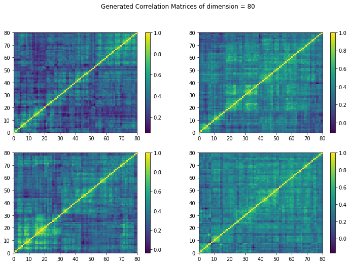
Here we show a sample of the type of empirical correlation matrices CorrGAN was trained on.

Figure 7. CorrGAN correlation matrices comparison.

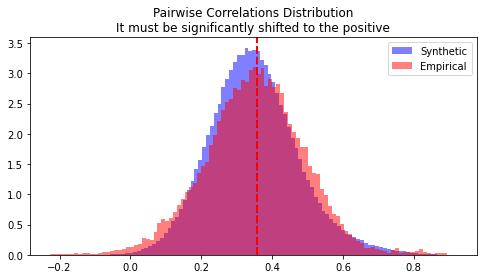
1. Distribution of pairwise correlations is significantly shifted to the positive

# Convert pandas dataframe to numpy array.
empirical_mats = []
for date, corr_mat in rolling_corr.groupby(level=0):
    empirical_mats.append(corr_mat.values)
empirical_mats = np.array(empirical_mats)

# Plot all stylized facts.
plot_stylized_facts(empirical_mats, corrgan_mats)

Figure 8 shows the positive shift to the right of the correlation factors is observed. Even though there are a few discrepancies in the tails of the empirical and generated distributions, this stylized factor holds true for both. Both have a mean value of around 0.37.

Figure 8. Pairwise correlation distributions comparison.

2. Eigenvalues follow the Marchenko-Pastur distribution, but for a very large first eigenvalue (the market).
3. and a couple of other large eigenvalues (industries)

In Figure 9, the distribution of eigenvalues closely matches the empirical and generated values. We observe a large first eigenvalue, followed for a few eigenvalues, larger than the remaining ones.

Figure 9. Mean eigenvalues distribution comparison.

4. Perron-Frobenius property (first eigenvector has positive entries).

From Figure 10, the distribution of the first eigenvector entries are all positive. Even though the empirical and generated data distributions do not closely match in magnitude, the Perron-Frobenius property holds true for both.

Figure 10. Mean first eigenvector distributions comparison.

5. Hierarchical structure of correlations. 

In figure 11 we observe hierarchical clustering for both the empirical and generated matrices. Note how dimensions 0-8 in the empirical matrix and the generated matrix exhibit similar, although of different magnitude, clusters. The dimensions 10 and onwards exhibit a similar clustering as well.

Figure 11. Hierarchical structure of correlation matrices. Top figure is the empirical matrix, the bottom figure is the synthetic matrix.

6. Scale-free property of the corresponding Minimum Spanning Tree (MST).

From Figure 12, we can observe that the MST distribution of node degrees conforms to the scale-free property (degree distribution follows a power law.) for both empirical and generated data.

Figure 12. Scale-free property of the MST comparison.

References:

- Abasi, B., Margenot, M. and Granizo-Mackenzie, D. (n.d.) The Capital Asset Pricing Model and Arbitrage Pricing Theory [Online]. Available at: https://www.quantopian.com/lectures/the-capital-asset-pricing-model-and-arbitrage-pricing-theory. (Accessed: 26 Aug 2020)
- Laloux, L., Cizeau, P., Potters, M. and Bouchaud, J.P., 2000. Random matrix theory and financial correlations. International Journal of Theoretical and Applied Finance, 3(03), pp.391-397.
- Hüttner, A., Mai, J., and Mineo, S., 2018. Portfolio selection based on graphs: Does it align with Markowitz-optimal portfolios?. Dependence Modeling, 6(1), pp.63-87
- Marti, G., 2020a, May. CorrGAN: Sampling Realistic Financial Correlation Matrices Using Generative Adversarial Networks. In ICASSP 2020-2020 IEEE International Conference on Acoustics, Speech and Signal Processing (ICASSP) (pp. 8459-8463). IEEE
- Marti, G. (2020b) TF 2.0 DCGAN for 100×100 financial correlation matrices [Online]. Available at: https://marti.ai/ml/2019/10/13/tf-dcgan-financial-correlation-matrices.html. (Accessed: 17 Aug 2020)
- Goodfellow, I., Pouget-Abadie, J., Mirza, M., Xu, B., Warde-Farley, D., Ozair, S., Courville, A. and Bengio, Y., 2014. Generative adversarial nets. In Advances in neural information processing systems (pp. 2672-2680).