Distance Approach in Pairs Trading: Part I

by Joohwan Ko

Join the Reading Group and Community: Stay up to date with the latest developments in Financial Machine Learning!

LEARN MORE ABOUT PAIRS TRADING STRATEGIES WITH “THE DEFINITIVE GUIDE TO PAIRS TRADING”

What is the Distance Approach?

There are many types of approaches you can use in pairs trading, but the Distance Approach is one of the most widely used because of its simplicity. The basic concept is as follows: Using Euclidean squared distance on the normalized price time series, $n$ closest pairs of assets are chosen as pairs.

$S S D=\sum_{t=1}^{N}\left(P_{t}^{1}-P_{t}^{2}\right)^{2}$

Then, with selected pairs, if the difference between the price of elements in a pair diverged by more than a threshold(ex. 2 standard deviations), the positions are opened. We have a long position for a stock with a lower price and a short position for a higher price in the portfolio.

Although as simple as it seems, the Distance Approach can have various pairs selection and portfolio formation strategies to the extent that it does not deviate significantly from its key concept. Here, in this blog post, we’ll look into four different pairs selection methods you can use in the Distance Approach. We’ll cover the advanced version of the Distance Approach in the following post – Introduction to Distance Approach in Pairs Trading: Part II.

Basic Distance Approach

Before we mainly dive into four different pairs selection methods, we’ll present the basic structure of the Distance Approach. There are two stages in the Distance Approach: pairs formation and trading signal generation. In the stage of pairs formation, these three steps need to be done in order to form pairs.

Normalization of the input data
Pairs selection
Calculating the historical volatility

First, we have to normalize the input data. The main reason for this is that as all of the stocks have different scales of prices, we need to uniform the scales to calculate the Euclidean distance in the pairs selection part. Any normalization method would be applied in this step, but usually, a min-max normalization is used.

$P_{\text {normalized }}=\frac{P-\min (P)}{\max (P)-\min (P)}$

Next is the pairs selection. As we’ll cover different pairs selection methods in the next chapter, you may think of the basic pairs selection method, which is done by calculating the Euclidean distance between stocks and selecting the closest pairs. Finally, we have to calculate the historical volatility of stocks in the formation period:

$\sigma = \sqrt{\frac{\sum_{t=1}^{N}\left(P_{t}-\bar{P}\right)^{2}}{N-1}}$

This step is necessary because the method uses this value as a threshold in the trading period.

Pairs Selection Methods

Four pairs selection methods are as follows:

Pairs with the smallest distance
Pairs within the same industry group
Pairs with a higher number of zero-crossings
Pairs with a higher historical standard deviation

Pairs with the smallest distance

This method is called the basic method and it is the one we covered in the Introduction part. Therefore, we’ll just move on to the next method.

Pairs within the same industry group

This method is a slight extension of the basic method. Instead of selecting pairs in the whole stock universe, this method selects pairs only within the same industry group. By calculating the Euclidean square distance for each pair within the same group, the n closest pairs are chosen.

Pairs with a higher number of zero-crossings

The concept of zero-crossings is very straightforward. Defined as the number of times the normalized spread crosses the value zero, it measures the frequency of divergence and convergence between two securities. Intuitively speaking, good candidates are those that not only track each other well (captured by the SSD metric) but also exhibit frequent deviations that are subsequently reversed under the force of arbitrage. This was even proved as statistically significant by the work of Do and Faff (2010). In the equation below, the estimated coefficients for the zero-crossings are statistically significant, which means that the higher the number of zero crossings, the higher chance of getting more pair returns.

$\begin{aligned}\text { Pair return }_{i}=& \text { Constant }+a_{1} \text { Time trend }+a_{2} \mathrm{SSD}_{i} \\&+a_{3} S S D_{i}^{2}+a_{4} \log (\text { Zero crossings }) \\&+a_{5} \text { SameIndustryFlag }+a_{6} \text { IndustryVol }_{i} \\&+a_{7}\left(\text { IndustryVol }_{i}\right)^{2}+e_{i},\end{aligned}$

Pairs with a higher historical standard deviation

This method was introduced due to some limitations of SSD. The equation below shows that constraining for low SSD is the same as minimizing the sum of (i) spread variance and (ii) squared spread mean. This selection metric is prone to form pairs with low spread variance, which ultimately limits profit potential and is in conflict with the objectives of a rational investor in pairs trading. Therefore, by adding the criteria of selecting pairs with a higher standard deviation, this method minimizes the limitations of the basic method.

$\overline{S S D_{i j t}}=\frac{1}{T} \sum_{t=1}^{T}\left(P_{i t}-P_{j t}\right)^{2}=\mathrm{V}\left(P_{i t}-P_{j t}\right)+\left(\frac{1}{T} \sum_{t=1}^{T}\left(P_{i t}-P_{j t}\right)\right)^{2}$

Trading Strategy

Portfolio Creation

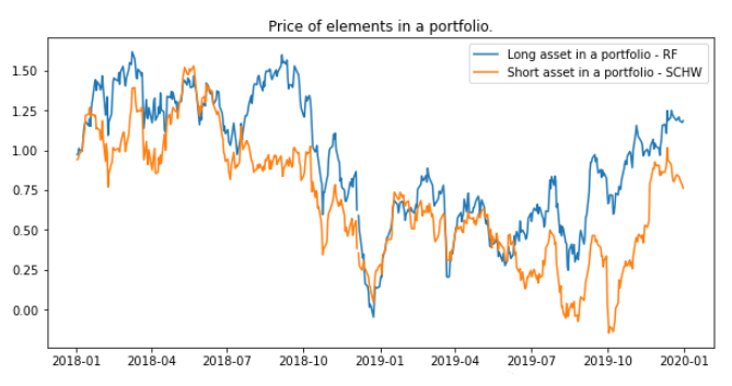
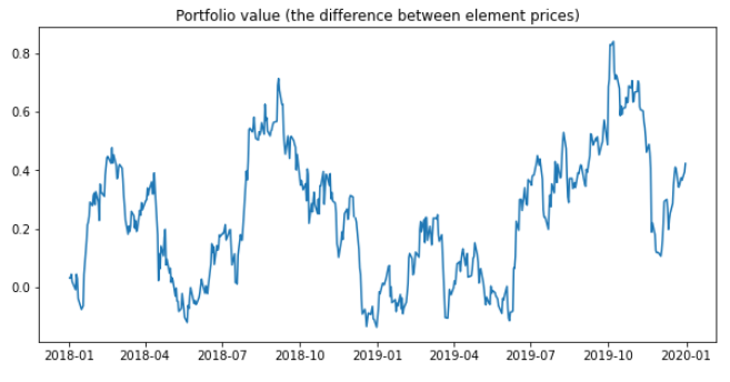
Now it’s time to trade with the pairs we created in the previous steps. In order to generate trading signals, we need another input data for trading period and normalize it in the same way we did in the formation period. After the data is preprocessed, the Distance Approach creates portfolios with the asset pairs. Portfolio values series are differences between normalized price series of elements in a pair as in the figure below. The first figure shows two different normalized price series of two stocks, and the second shows the portfolio price series.

Fig. 1: Plot of two price series of stocks.

Fig. 2: Plot of portfolio price series.

Generating Trading Signals

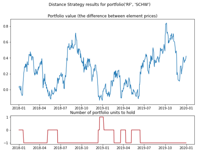
After the portfolio is created, the Distance Approach generates trading signals for the last step of pairs trading. First, we need to set a threshold. This is a threshold to enter a position for pairs portfolios and is usually set around two standard deviations. If the portfolio value exceeds the threshold, a sell signal is generated – we expect the price of the first element to decrease and the price of the second element to increase. And if the value of the portfolio is below a minus threshold, a buy signal is generated. Here’s an example of trading signals for a pair:

Fig. 3: Plot of portfolio prices series and its generated trading signals.

After the trading signals are generated, you can use these signals for pairs trading!

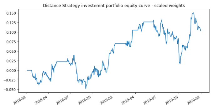
Equity curve generated used trading signalsrading signals

Fig. 4: Equity curve generated using trading signals.

Possible Improvements

Although it is widely used due to its simplicity, there are some limitations to the Distance Approach.

Pairs are selected only based on a pair of two stocks without considering others.
Only the price movement of two stocks is considered in generating trading signals.
Once pairs are selected in the formation period, no other stocks are considered to be traded in the trading period, which may miss some possible opportunities for profits.

A lot of research has been conducted to solve these problems, and some of the advanced Distance Approach is as follows:

Apply quasi-multivariate approach both in selecting pairs and generating trading signals
Apply different pairs selection method such as Pearson Correlation
Consider the whole universe of stocks in each timestamp of the trading period not to miss any chance of profits

We’ll cover the advanced Distance Approach in the following post so stay tuned if you are interested!

References

- Krauss, C., 2017. Statistical arbitrage pairs trading strategies: Review and outlook. Journal of Economic Surveys, 31(2), pp.513-545.
- Gatev, E., Goetzmann, W.N. and Rouwenhorst, K.G., 2006. Pairs trading: Performance of a relative-value arbitrage rule. The Review of Financial Studies, 19(3), pp.797-827.
- Do, B. and Faff, R., 2010. Does simple pairs trading still work?. Financial Analysts Journal, 66(4), pp.83-95
- Do, B. and Faff, R., 2012. Are Pairs Trading Profits Robust to Trading Costs?. SSRN Electronic Journal.