Previously Proposed Approaches

Pairs trading methods differ in how they form pairs, the trading rules used, or both. The dominating non-parametric method was published in the landmark paper of Gatev et al: “Pairs trading: Performance of a relative-value arbitrage rule”, where they propose using a distance-based approach to select the securities for constructing the pairs. The criterion used was choosing pairs that minimized the sum of squared deviations between the two normalized prices. They argue that this approach “best approximates the description of how traders themselves choose pairs”.

Overall, the nonparametric distance-based approach provides a simple and general method of selecting “good” pairs, however, this selection metric is prone to pick up pairs with a small amount of variance of the spread and therefore limits overall profitability.

Another two popular approaches are the cointegration and correlation methods. Basically, correlation reflects short-term linear dependence in returns while on the other hand cointegration models long-term dependencies in prices (Alexander 2001).

A significant issue with the correlation approach is that two securities correlated on a returns level do not necessarily share an equilibrium relationship, and there is no theoretical foundation that divergences are reversed. This potential lack of an equilibrium relationship leads to higher divergence risks and thus to significant potential losses.

High correlations may well be spurious since high correlation is not related to a cointegration relationship (Alexander 2001). Omitting cointegration testing is very much contradictory to the requirements of a rational investor.

The Problem of Multiple Hypothesis Testing

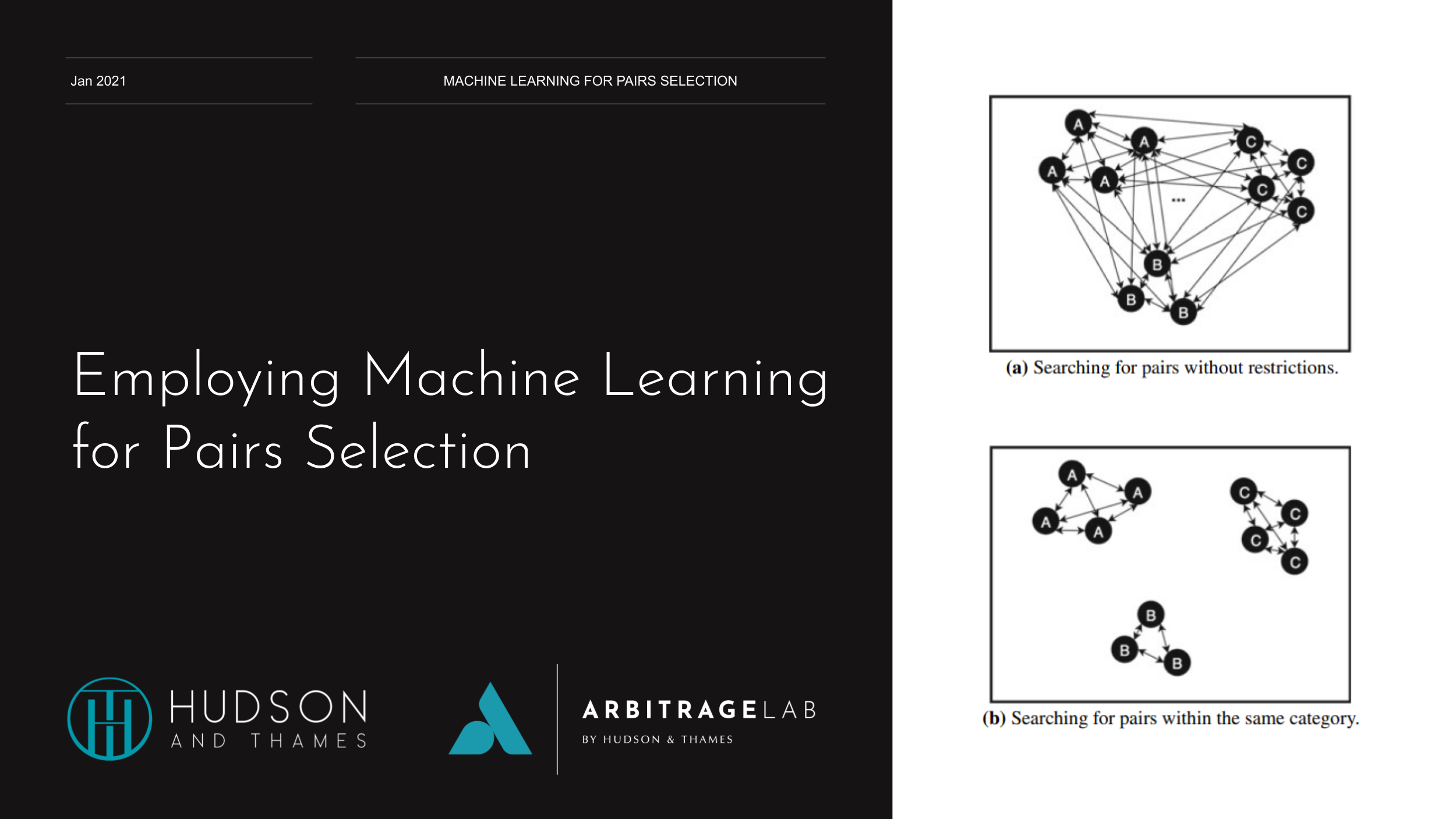
As the popularity of Pairs Trading grows, it is increasingly harder to find rewarding pairs. The simplest procedure commonly applied is to generate all possible candidate pairs by considering the combination from every security to every other security in the dataset.

Two different problems arise immediately.

First, the computational cost of testing mean-reversion for all the possible combinations increases drastically as more securities are considered.

The second emerging problem is frequent when performing multiple hypothesis tests at once and is referred to as the multiple comparisons problem. By definition, if 100 hypothesis tests are performed (with a confidence level of 5%) the results should contain a false positive rate of 5%.

This problem was tackled by (Harlacher 2016), who found that Bonferroni correction leads to a very conservative selection of pairs and impedes the discovery of even truly cointegrated combinations. The paper recommends the effective pre-partitioning of the considered asset universe to reduce the number of feasible combinations and, therefore, the number of statistical tests. This aspect might lead the investor to pursue the usual, more restrictive approach of comparing securities only within the same sector.

This dramatically reduces the number of necessary statistical tests, consequently decreasing the likelihood of finding spurious relations. However, the simplicity of this process might also turn out to be a disadvantage. The more traders are aware of the pairs, the harder it is to find pairs not yet being traded in large volumes, leaving a smaller margin for profit.

This dilemma motivated the work of (Sarmento and Horta 2020) in the search for a methodology that lies in between these two scenes: an effective pre-partitioning of the universe of assets that does not limit the combination of pairs to relatively obvious solutions, while not enforcing excessive search combinations.

How can Machine Learning solve this?

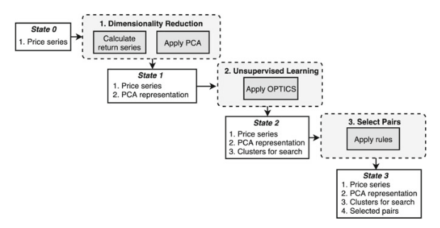
In this work (Sarmento and Horta 2020), propose a three-pronged process, built using unsupervised learning algorithms, on the expectation that it infers meaningful clusters of assets from which to select the pairs.

Figure 1: Proposed Framework diagram from (Sarmento and Horta 2020).

The premise is to extract empirical structure that the data is manifesting, rather than imposing fundamental groups each security should belong to. The proposed methodology encompasses the following steps:

1. Dimensionality reduction – find a compact representation for each security;
2. Unsupervised Learning – apply an appropriate clustering algorithm;
3. Select pairs – define a set of rules (ARODS) to select pairs for trading.

Dimensionality Reduction

Dimensionality reduction is the transformation of high-dimensional data into a meaningful representation of reduced dimensionality. It is important in many domains since it mitigates the curse of dimensionality and other undesired properties of high-dimensional spaces. Ideally, the reduced representation should have a dimensionality that corresponds to the intrinsic dimensionality of the data. The intrinsic dimensionality of data is the minimum number of parameters needed to account for the observed properties of the data.

In the quest for profitable pairs, we wish to find securities with the same systematic risk-exposure. Any deviations from the theoretical expected return can thus be seen as mispricing and serve as a guideline to place trades. The application of PCA on the return series is proposed to extract the common underlying risk factors for each security, as described in (Avellaneda and Lee 2010).

PCA is a statistical procedure that uses an orthogonal transformation to convert a set of observations of possibly correlated variables into a set of linearly uncorrelated variables, the principal components. The transformation is defined such that the first principal component accounts for as much of the variability in the data as possible. Each succeeding component, in turn, has the highest variance possible under the constraint that it must be orthogonal to the preceding components.

Clustering

There exist several unsupervised learning clustering techniques capable of solving the task at hand. Two main candidates are showcased: DBSCAN and OPTICS.

DBSCAN, as the name implies, is a density-based clustering algorithm, which given a set of points in some space, it groups together points that are closely packed together.

OPTICS is an extension built upon the idea of DBSCAN, but improves on its major weakness: the problem of detecting meaningful clusters in data of varying density. To do so, the points of the database are ordered such that spatially closest points become neighbors in the ordering. Additionally, a special distance is stored for each point that represents the density that must be accepted for a cluster so that both points belong to the same cluster.

In summary, there are a few differences:

• Memory Cost: OPTICS requires more memory as it maintains a priority queue to determine the next data point which is closest to the point currently being processed in terms of reachability distance. It also requires more computational power because the nearest neighbor queries are more complicated than radius queries in DBSCAN.
• Fewer Parameters: OPTICS does not need to maintain the epsilon parameter making it relatively insensitive to parameter settings. Thus also leading to the reduction of manual parameter tuning.
• Interpretable: OPTICS does not segregate the given data into clusters. It merely produces a distance plot and it is upon the interpretation of the programmer to cluster the points accordingly.

The framework described till now has been implemented as a part of the ArbitrageLab library that has been in development for the last few months. The steps above have been condensed down into a simple manner as follows;

# Importing packages
import pandas as pd
import numpy as np
from arbitragelab.ml_approach import PairsSelector

# Getting the dataframe with time series of asset returns.
data = pd.read_csv('X_FILE_PATH.csv', index_col=0, parse_dates = [0])

ps = PairsSelector(data)

# Price data is reduced to its component features using PCA.
ps.dimensionality_reduction_by_components(5)

# Clustering is performed over the feature vector.
ps.cluster_using_optics({'min_samples': 3})

# Plot clustering results.
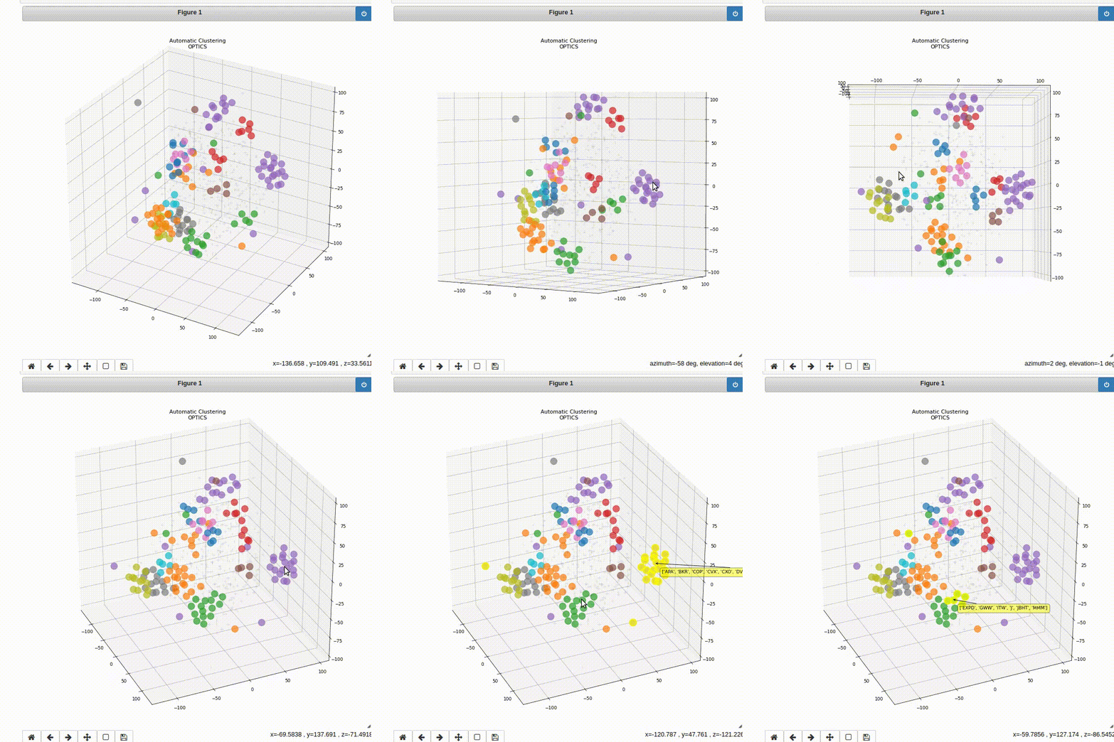
ps.plot_clustering_info(method='OPTICS', n_dimensions=3)

Figure 2: 3D plot of the clustering result using the OPTICS method.

Absolute Rules of Disqualification (ARODs)

The classical pairs selection approach encompasses two steps:

• Finding the appropriate candidate pairs and
• Selecting the most promising ones.

Having generated the clusters of assets in the previous steps, it is still necessary to define a set of conditions for selecting the pairs to trade. The most common approaches to select pairs are the distance, cointegration, and correlation approaches. The cointegration approach was selected because the literature suggests that it performs better than minimum distance and correlation approaches.

The selection process starts with the testing of pairs, generated from the clustering step, for cointegration using the Engle-Granger test. This cointegration testing method was chosen based on its simplicity. If you want to learn more about cointegration methods I recommend reading our article: An Introduction to Cointegration for Pairs Trading.

Figure 3: Pairs Selection Rules diagram from (Sarmento and Horta 2020).

Secondly, a validation step is implemented to provide more confidence in the mean-reversion character of the pairs’ spread. The condition imposed is that the Hurst exponent associated with the spread of a given pair is enforced to be smaller than 0.5, assuring the process leans towards mean-reversion. The Hurst exponent is a measure that quantifies the amount of memory in a specific time series, which in this case means, how mean-reverting is the process under analysis?

In third place, the pair’s spread movement is constrained using the half-life of the mean-reverting process. The half-life is the time that the spread will take to mean-revert half of its distance after having diverged from the mean of the spread, given a historical window of data. In the framework paper, the strategy built on top of the selection framework is based on the medium-term price movements, so for this reason the spreads that either have very short (< 1 day) or very long mean-reversion (> 365 days) periods are not suitable.

Lastly, every spread is checked to make sure it crosses its mean at least twelve times a year, to provide enough liquidity and thus providing enough opportunities to exit a position.

This step can be easily done writing the following lines of code;

# Generated Pairs are processed through the rules mentioned above
ps.unsupervised_candidate_pair_selector()

# Generate a Panel of information of the selected pairs
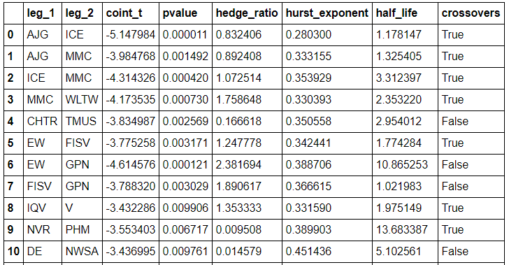
final_pairs_info = ps.describe_extra()

Conclusion

The success of a Pairs Trading strategy highly depends on finding the right pairs. The classical approaches to find tradable opportunities used by investors are either too restrictive, like restricting the search to inter-sector relationships, or too open, like removing any limit on the search space.

In this post, a Machine Learning based framework is applied to provide a balanced solution to this problem. Firstly with the application of unsupervised learning to define the search space. Secondly, in the grouping of relevant securities (not necessarily from the same sector) in clusters, and finally in the detection of rewarding pairs within them, that would otherwise be hard to identify, even for the experienced investor.

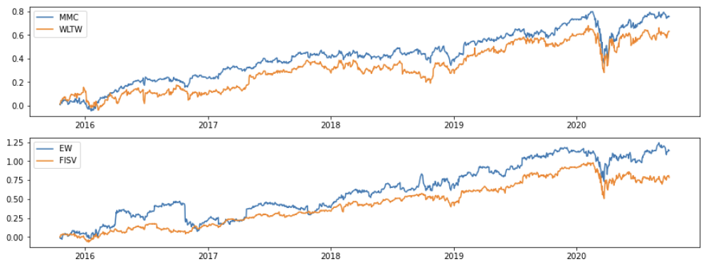
Figure 4: Example pairs found using the ArbitrageLab framework implementation.

Check out our lecture on the topic:

References

- Ankerst, M., Breunig, M.M., Kriegel, H.P., and Sander, J., 1999. OPTICS: ordering points to identify the clustering structure. ACM Sigmod Record, 28 (2), pp.49-60.
- Avellaneda, M. and Lee, J.H., 2010. Statistical arbitrage in the US equities market. Quantitative Finance, 10 (7), pp.761-782.
- Alexander, C., 2001. Market models. A Guide to Financial Data Analysis, 1.
- Gatev, E., Goetzmann, W.N. and Rouwenhorst, K.G., 2006. Pairs trading: Performance of a relative-value arbitrage rule. The Review of Financial Studies, 19(3), pp.797-827.
- Harlacher, M., 2016. Cointegration based algorithmic pairs trading. PhD thesis, University of St. Gallen.
- Maddala, G.S., and Kim, I.M., 1998. Unit roots, cointegration, and structural change (No. 4). Cambridge university press.
- Ramos-Requena, J.P., Trinidad-Segovia, J.E. and Sánchez-Granero, M.Á., 2020. Some Notes on the Formation of a Pair in Pairs Trading. Mathematics, 8 (3), p.348.
- Sarmento, S.M. and Horta, N., 2020. Enhancing a Pairs Trading strategy with the application of Machine Learning. Expert Systems with Applications, p.113490.
- Van Der Maaten, L., Postma, E., and Van den Herik, J., 2009. Dimensionality reduction: a comparative. J Mach Learn Res, 10 (66-71), p.13.