And now, we have two options: memorize everything or constantly switch between numerous parameters and plots to check, contrast and compare. It results in loading your brain with tons of ‘noise’ that distracts from focusing on the evaluation itself. But it doesn’t have to be this way. Data analysis thrives when there is order, accessibility and clarity. And what embodies these three qualities better than combining everything into an interactive well-rounded tear sheet? 

Introducing Arbitragelab TearSheets

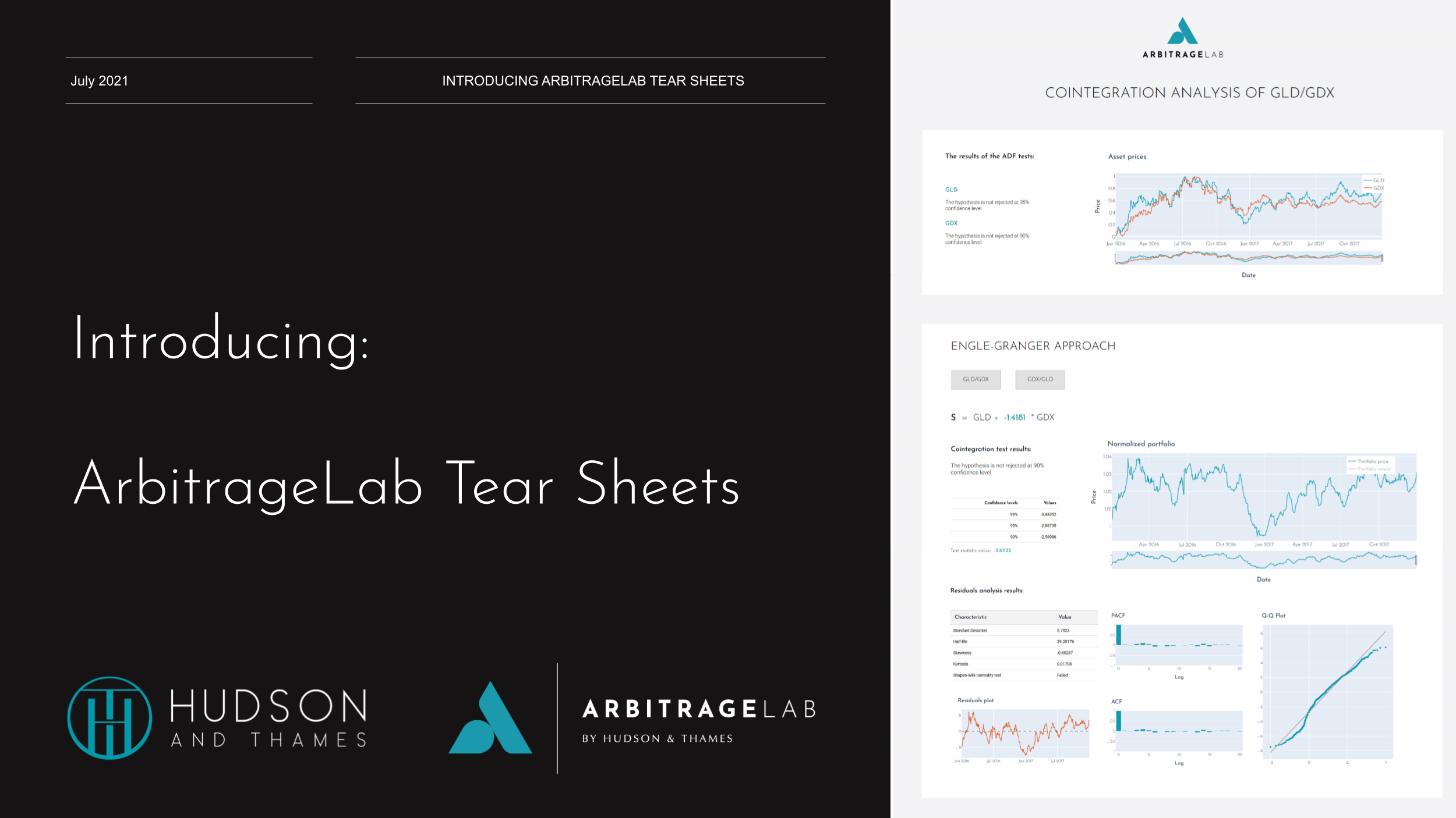
 Arbitragelab TearSheets is a new module created by the Hudson & Thames team that provides an interactive and effortless approach to pairs analysis. 

It provides two comprehensive tear sheet types: Cointegration analysis and OU model analysis, based on the most popular ArbitrageLab modules functionality. All you need is just a dataframe of asset prices. The module creates a locally run Flask server that hosts your interactive tear sheet and allows you to interact with it freely inside your browser or inside of your Jupyter Notebook if you wish so.

Import the module, load your data, and run the server. The process is as easy as 1, 2, 3. 

# Import the module
from arbitragelab.tearsheet.tearsheet import TearSheet

# Initialize the server
tearsheet = TearSheet()

server = tearsheet.ou_tearsheet(data)

# Run the server
server.run_server(port=8050)

Let’s dive a bit deeper into the mentioned tear sheets.