Meta Labeling (A Toy Example)

This blog post investigates the idea of Meta Labeling and tries to help build an intuition for what is taking place. The idea of meta labeling is first mentioned in the textbook Advances in Financial Machine Learning by Marcos Lopez de Prado and promises to improve model and strategy performance metrics by helping to filter-out false positives.

In this blog post we make use of a computer vision problem known as the MNIST handwritten digit classification. By making use of a non financial time series data set we can illustrate the components that make up meta labeling more clearly. Lets begin!

The following section is taken directly from the textbook and left in its original form as to make sure no errors are introduced by means of interpretation.

Advances in Financial Machine Learning, Chapter 3, page 50. Reads:

Suppose that you have a model for setting the side of the bet (long or short). You just need to learn the size of that bet, which includes the possibility of no bet at all (zero size). This is a situation that practitioners face regularly. We often know whether we want to buy or sell a product, and the only remaining question is how much money we should risk in such a bet. We do not want the ML algorithm to learn the side, just to tell us what is the appropriate size. At this point, it probably does not surprise you to hear that no book or paper has so far discussed this common problem. Thankfully, that misery ends here.

I call this problem meta labeling because we want to build a secondary ML model that learns how to use a primary exogenous model.

The ML algorithm will be trained to decide whether to take the bet or pass, a purely binary prediction. When the predicted label is 1, we can use the probability of this secondary prediction to derive the size of the bet, where the side (sign) of the position has been set by the primary model.

How to use Meta Labeling

Binary classification problems present a trade-off between type-I errors (false positives) and type-II errors (false negatives). In general, increasing the true positive rate of a binary classifier will tend to increase its false positive rate. The receiver operating characteristic (ROC) curve of a binary classifier measures the cost of increasing the true positive rate, in terms of accepting higher false positive rates.

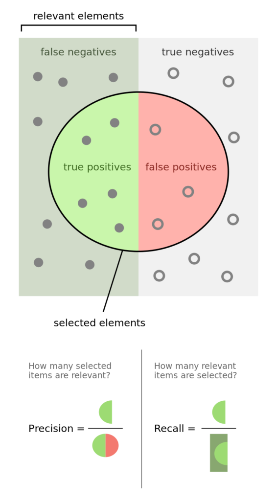
Figure 1: Precision and Recall

Wikipedia, the free encyclopedia 2019

The image illustrates the so-called “confusion matrix.” On a set of observations, there are items that exhibit a condition (positives, left rectangle), and items that do not exhibit a condition (negative, right rectangle). A binary classifier predicts that some items exhibit the condition (ellipse), where the TP area contains the true positives and the TN area contains the true negatives. This leads to two kinds of errors: false positives (FP) and false negatives (FN). “Precision” is the ratio between the TP area and the area in the ellipse. “Recall” is the ratio between the TP area and the area in the left rectangle. This notion of recall (aka true positive rate) is in the context of classification problems, the analogous to “power” in the context of hypothesis testing. “Accuracy” is the sum of the TP and TN areas divided by the overall set of items (square). In general, decreasing the FP area comes at a cost of increasing the FN area, because higher precision typically means fewer calls, hence lower recall. Still, there is some combination of precision and recall that maximizes the overall efficiency of the classifier. The F1-score measures the efficiency of a classifier as the harmonic average between precision and recall.

Meta labeling is particularly helpful when you want to achieve higher F1-scores. First, we build a model that achieves high recall, even if the precision is not particularly high. Second, we correct for the low precision by applying meta labeling to the positives predicted by the primary model.

Meta labeling will increase your F1-score by filtering out the false positives, where the majority of positives have already been identified by the primary model. Stated differently, the role of the secondary ML algorithm is to determine whether a positive from the primary (exogenous) model is true or false. It is not its purpose to come up with a betting opportunity. Its purpose is to determine whether we should act or pass on the opportunity that has been presented.

Additional uses of Meta Labeling

Meta labeling is a very powerful tool to have in your arsenal, for four additional reasons. First, ML algorithms are often criticized as black boxes.

Meta labeling allows you to build an ML system on top of a white box (like a fundamental model founded on economic theory). This ability to transform a fundamental model into an ML model should make meta labeling particularly useful to “quantamental” firms. Second, the effects of overfitting are limited when you apply meta labeling, because ML will not decide the side of your bet, only the size. Third, by decoupling the side prediction from the size prediction, meta labeling enables sophisticated strategy structures. For instance, consider that the features driving a rally may differ from the features driving a sell-off. In that case, you may want to develop an ML strategy exclusively for long positions, based on the buy recommendations of a primary model, and an ML strategy exclusively for short positions, based on the sell recommendations of an entirely different primary model. Fourth, achieving high accuracy on small bets and low accuracy on large bets will ruin you. As important as identifying good opportunities is to size them properly, so it makes sense to develop an ML algorithm solely focused on getting that critical decision (sizing) right. In my experience, meta labeling ML models can deliver more robust and reliable outcomes than standard labeling models.

Toy Example

To illustrate the concept we made use of the MNIST data set to train a binary classifier on identifying the number 3, from a set that only includes the digits 3 and 5. The reason for this is that the number 3 looks very similar to 5 and we expect there to be some overlap in the data, i.e. the data are not linearly separable. Another reason we chose the MNIST dataset to illustrate the concept, is that MNIST is a solved problem and we can witness improvements in performance metrics with ease.

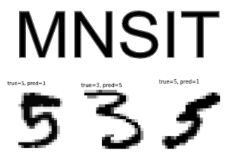
Figure 2: Handwritten 5 and 3

Model Architecture

The following image explains the model architecture. The first step is to train a primary model (binary classification) with a high recall. Second a threshold level is determined at which the primary model has a high recall, ROC curves could be used to help determine a good level. Third the features from the first model are concatenated with the predictions from the first model, into a new feature set for the secondary model. Meta labels are used as the target variable in the second model. Now fit the second model. Fourth the prediction from the secondary model is combined with the prediction from the primary model and only where both are true, is your final prediction true. I.e. if your primary model predicts a 3 and your secondary model says you have a high probability of the primary model being correct, is your final prediction a 3, else not 3.

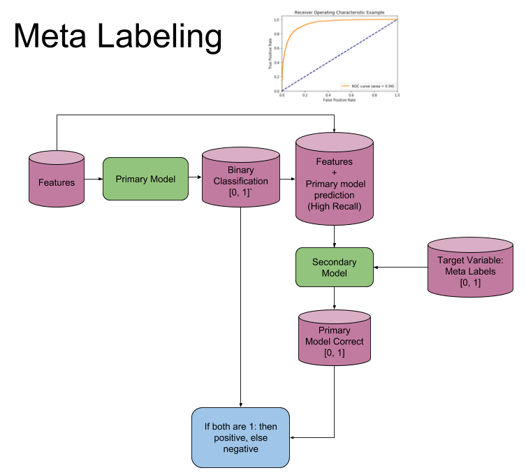
Figure 3: Meta Label Model Architecture

Build Primary Model with High Recall

The first step is to train a primary model (binary classification). For this we trained a logistic regression, using the keras package. The data are split into a 90\% train, 10\% validation. This allows us to see when we are over-fitting.

Second a threshold level is determined at which the primary model has a high recall, ROC curves could be used to help determine a good level. A high recall means that the primary model captures the majority of positive samples even if there are a large number of false positives. The meta model will correct this by reducing the number of false positives and thus boosting all performance metrics.

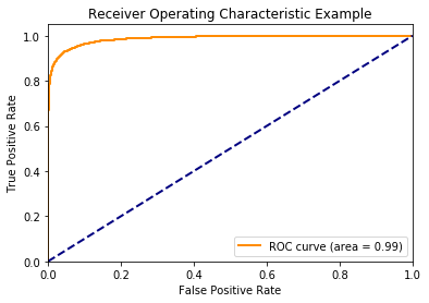
Figure 4: Receiver Operating Characteristic (ROC) Curve

Build Meta Model

Third the features from the first model are concatenated with the predictions from the first model, into a new feature set for the secondary model. Meta labels are used as the target variable in the second model. Now fit the second model.

Meta labels are defined as: If the primary model’s predictions matches the actual values, then we label it as 1, else 0. In this example we said that if an observation was a true positive or true negative then label it as 1(i.e. the model is correct), else 0 (the model in incorrect). Note that because it is categorical, we have to add One Hot Encoding.

Evaluate Performance

Fourth the prediction from the secondary model is combined with the prediction from the primary model and only where both are true, is your final prediction true. e.g. if your primary model predicts a 3 and your secondary model says you have a high probability of the primary model being correct, is your final prediction a 3, else not a 3.

The section below shows the performance of the primary model vs the performance of using Meta labeling, on out-of-sample data. Notice how the performance metrics improve.

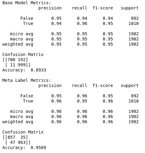
Figure 5: Meta Labeling Performance Metrics

We can see that in the confusion matrix, that the false positives from the primary model, are now being correctly identified as true negatives with the help of meta labeling. This leads to a boost in performance metrics. Meta labeling works as advertised!

To read more about meta labeling used in a trading strategy (Trend following and Mean reverting), be sure to checkout our article titled: Does Meta Labeling Add to Signal Efficay?