Minimum Profit Optimization: Mean-reversion Trading

Minimum Profit Optimization: Optimal Boundaries for Mean-reversion Trading

by Yefeng Wang

Join the Reading Group and Community: Stay up to date with the latest developments in Financial Machine Learning!

LEARN MORE ABOUT PAIRS TRADING STRATEGIES BY JOINING OUR NEWSLETTER

Introduction

In my previous articles, I introduced how to construct long-short asset pairs according to the concept of cointegration and how to build a sparse mean-reverting multi-asset portfolio. Now that we are able to answer the question “what to trade” with confidence, it is time to get down to the nitty-gritty of the implementation of a mean-reversion strategy.

The crux of implementing a mean-reversion trading strategy is to pinpoint the trade location. Apparently, we want to initiate a trade when the spread value has deviated considerably from its long-term mean. However, “a considerable deviation” is a rather vague description and needs to be quantified when it comes to trade execution. For the sake of convenience and clarity, I will use “boundary” to refer to the trade location and “spread” to both the spread of the long-short asset pairs and the value of the multi-asset portfolio in the remainder of this article.

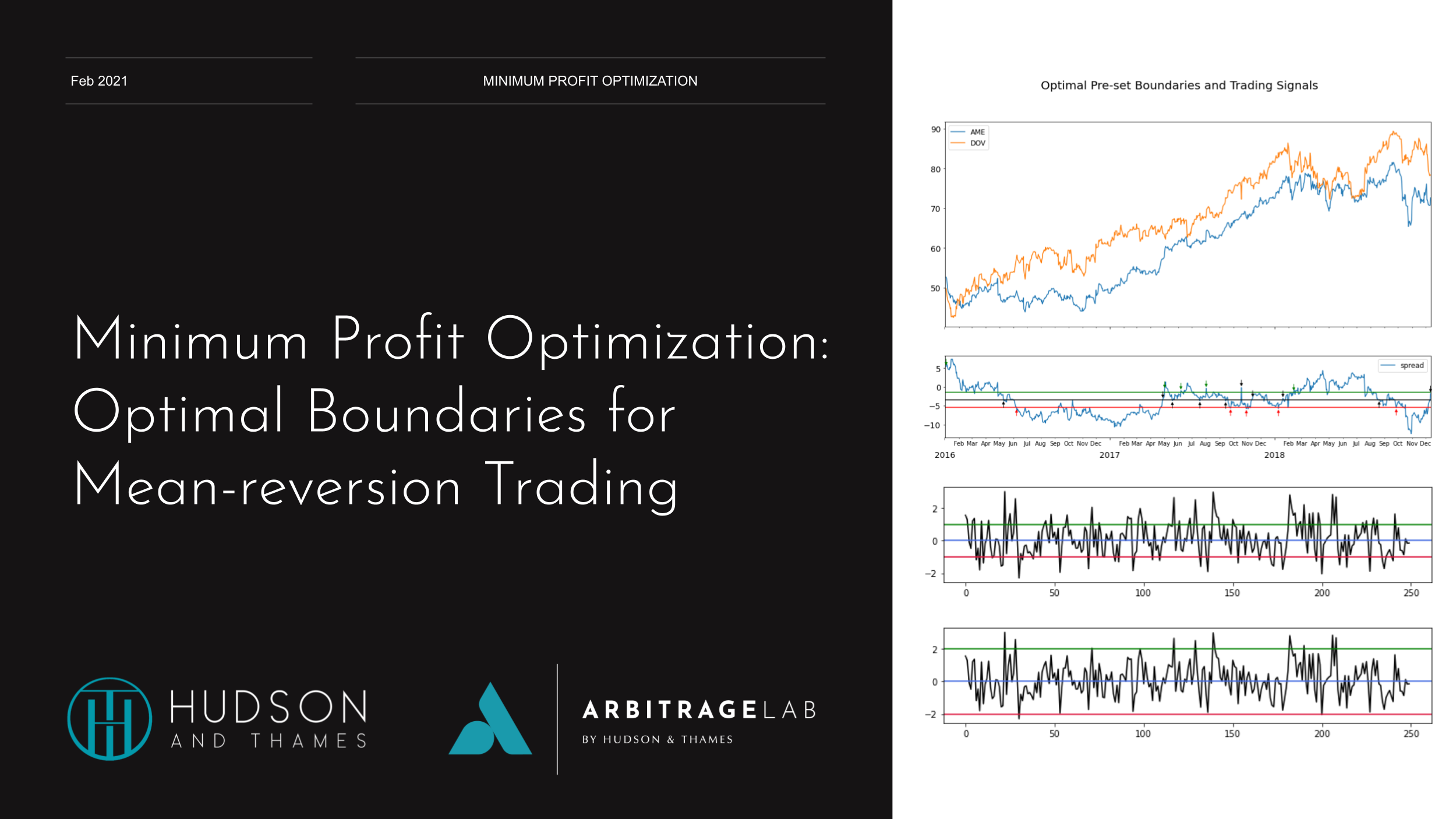
Figure 1. Two mean-reversion strategies with different trade locations on the same simulated stationary AR(1) series.

Let’s use a toy example to illustrate the importance of the boundaries. The trading strategy is rather simple: we initiate a short position when the spread value is above the upper boundary (green line) and a long position when the spread value is below the lower boundary (red line). The exit condition is the same: when the spread value returns to the mean (blue line), the position is closed.

The only difference between the two strategies is the location of the boundaries. The first strategy set the boundaries at $\pm1$ . The boundaries are tight, which make the strategy trade frequently, but each trade yields a smaller minimum profit. The second strategy set a wider boundaries at $\pm2$ . Now the trades are far less frequent, but each trade yields a greater minimum profit. The boundaries effectively governs the tradeoff between trade frequency versus the minimum profit per trade.

A tradeoff implies that an optimization opportunity is just around the corner. “Sweet spots” for both boundaries should exist such that the minimum total profit over a defined time period, which is just the minimum profit per trade multiplied by the number of trades, is maximized. This article will demonstrate how to formulate and solve this optimization problem using the concept of mean first-passage time of a stationary AR(1) process based on the work of Puspaningrum, Lin, and Gulati (2009).

Mean First-passage Time of a Stationary AR(1) process

What exactly is the first-passage time of a process? Its rigorous mathematical definition looks rather daunting, but let’s take a peek anyway. The first-passage time of a process $Z_t$ passing through a lower boundary $a$ is defined as follows:

$\mathcal{T}_a(z_0) = \mathcal{T}_{a,\infty}(z_0) = \inf \{t: Z_t < a \vert Z_0 = z_0 \geq a \}$

Similarly, the first-passage time of the same process passing through a upper boundary $b$ is defined as follows:

$\mathcal{T}_b(z_0) = \mathcal{T}_{-\infty, b}(z_0) = \inf \{t: Z_t > b \vert Z_0 = z_0 \leq b \}$

While looking rather intricate, these equations can still be translated into plain English. Let’s take the first equation as an example. The first-passage time of $Z_t$ through the lower boundary $a$ is only defined when $Z_t$ has an initial value greater than $a$ . When this condition is satisfied, we can simply take the earliest time when the value of $Z_t$ goes below $a$ . The first-passage time through the upper boundary $b$ can be explained likewise.

Still confused? Don’t worry, I have prepared a visualized explanation.

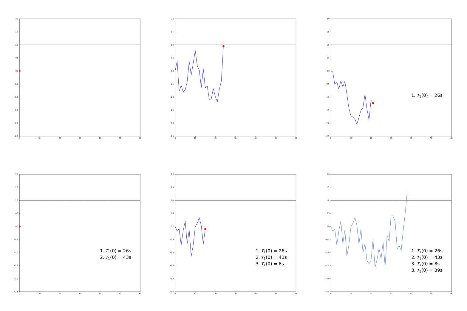
Figure 2. An animated demonstration of first-passage time. All four time series are simulated with a stationary AR(1) process (The AR(1) coefficient is 0.9) and starts at $z_0 = 0$ . The time elapsed after they first pass through the upper boundary, which is $b = 1.0$ in this example, has been recorded. The corresponding notation is thus $\mathcal{T}_1(0)$ .

Hope this animated example has helped you understand the concept of first-passage time. So why is first-passage time important?

The first-passage time can help us determine the trade frequency. Let’s say we initiated a trade exactly at the upper boundary. As soon as the spread crosses over the mean for the first time, we will close the trade without hesitation. This matches the definition of first-passage time perfectly. If we can get a reliable estimate of how long this crossover would happen on average, we know the expected trade duration. Similarly, we can also estimate the expected duration of the spread that starts at the long-term mean crossing over the upper boundary. This corresponds to how long we need to wait to put on a position, i.e. the expected inter-trade interval. With both the expected trade duration and inter-trade interval known, we can easily calculate the expected number of trades within a certain time period.

We can see from Figure 2 that the first-passage time is highly variable. The shortest first-passage time was only 8 seconds, while the longest first-passage time was 43 seconds, a 5.4 times difference. When it comes to strategy execution, we need to obtain an estimate of the expected first-passage time on average as we cannot rely on previous observations of first-time passages. The first-passage time is influenced by a few factors:

The property of the time series itself, e.g. stationarity.
The starting location of the time series.
The location of the boundary.

The first factor is crucial. The first-passage time might be intractable if the time series is ill-behaved. Fortunately, since our focus is on mean-reversion trading strategies, it is thus safe to assume stationarity of the spread, which is guaranteed by construction via either cointegration tests or sparse mean-reverting portfolio selection methods. Furthermore, we assume the spread follows an AR(1) process as its mean first-passage time is tractable and can be numerically estimated.

I will directly give the formula of the mean first-passage time of a stationary AR(1) process.

$E(\mathcal{T}_{a,b}(z_0)) = \frac{1}{\sqrt{2\pi}\sigma} \int_a^b E(\mathcal{T}_{a,b}(u)) \exp \Big(- \frac{(u-\phi z_0)^2}{2\sigma^2} \Big) du + 1$

where $\phi$ and $\sigma$ are defined by the stationary AR(1) process:

$Z_t = \phi Z_{t-1} + \xi_t$
$\vert \phi \vert < 1$
$\xi_t \sim N(0, \sigma^2) \; \text{i.i.d}$

Curious readers can find the derivation in Basak and Ho (2004).

Calculating Mean First-passage time of a Stationary AR(1) Process

I will briefly go over the numerical methods to obtain a reasonable estimate for $E(\mathcal{T}_{a,b}(z_0))$ for completeness. If you are more interested in the application of this method rather than the technical details, you can skip this part.

Notice that there is a similar term $E(\mathcal{T}_{a,b}(u))$ in the integral on the other side of the formula. Therefore, the first step is to use trapezoidal rule to convert the integral into a summation.

$\begin{align*} E(\mathcal{T}_{a,b}(z_0)) & = \frac{1}{\sqrt{2\pi}\sigma}\int_a^b E(\mathcal{T}_{a,b}(u)) \exp \Big( -\frac{(u-\phi z_0)^2}{2\sigma^2} \Big)du + 1 \\ &= \frac{h}{2\sqrt{2\pi}\sigma}\sum_{j=0}^n w_j E(\mathcal{T}_{a,b}(u_j)) \exp \Big( -\frac{(u_j - \phi z_0)^2}{2\sigma^2} \Big) +1 \end{align*}$

where $h = \frac{b-a}{n}$ , $n$ is the number of partitions in $[a,b]$ and $h$ is the length of each partition. The higher the $n$ , the finer each slice of the partition $[a,b]$ is, and the more exact the final estimation will be. Moreover, according to trapezoidal rule, the values of $w_j$ are as follows:

$w_j = \begin{cases} 1 \quad & \text{for } j = 0 \text{ or } j = n \\ 2 \quad & \text{otherwise } \end{cases}$

There are $n+1$ grid points $u_j$ for $n$ intervals, the idea here is thus to evaluate the summation at each grid point to get a linear system of $n+1$ equations with respect to $n+1$ variables, which

Denote

$K(u_i, u_j) = \frac{h}{2\sqrt{2\pi}\sigma}w_j \exp \Big( -\frac{(u_j - \phi u_i)^2}{2\sigma^2} \Big)$

Then the linear system can be written as

$\begin{pmatrix} 1 - K(u_0, u_0) & -K(u_0, u_1) & \ldots & -K(u_0, u_n) \\ -K(u_1, u_0) & 1 - K(u_1, u_1) & \ldots & -K(u_1, u_n) \\ \vdots & \vdots & \vdots & \vdots \\ -K(u_n, u_0) & -K(u_n, u_1) & \ldots & 1-K(u_n, u_n) \end{pmatrix} \begin{pmatrix} E_n(\mathcal{T}_{a,b}(u_0)) \\ E_n(\mathcal{T}_{a,b}(u_1)) \\ \vdots \\ E_n(\mathcal{T}_{a,b}(u_n)) \\ \end{pmatrix} = \begin{pmatrix} 1 \\ 1 \\ \vdots \\ 1 \\ \end{pmatrix}$

This can be readily solved in $O(n^3)$ time.

Getting the Estimates of Trade Duration and Inter-trade Interval

Now that we have a working numerical algorithm to calculate mean first-passage time of a stationary AR(1) series, we can obtain estimates of trade duration and inter-trade interval. Recall the definition of trade duration and inter-trade interval based on mean first-passage time:

Trade duration ( $TD(U)$ ): Average time elapsed between the time series starting at the upper boundary $U$ and crossing over its mean.
Inter-trade interval ( $I(U)$ ): Average time elapsed between the time series starting at its mean and crossing over the upper boundary $U$ .

The case for lower boundary is the same due to symmetry, for the mean of the spread will be always centered to zero before any calculation.

Substituting the upper boundary $U$ and the mean (which is zero) into the mean first-passage time equation and we can obtain:

$TD(U) = E(\mathcal{T}_{0, \infty}(U)) = \lim_{b \to \infty} \frac{1}{\sqrt{2 \pi} \sigma} \int_0^b E(\mathcal{T}_{0, b}(s)) \> \mathrm{exp} \Big( - \frac{(s- \phi U)^2}{2 \sigma^2} \Big) ds + 1$

$I(U) = E(\mathcal{T}_{- \infty, U}(0)) = \lim_{-b \to - \infty} \frac{1}{\sqrt{2 \pi} \sigma} \int_{-b}^U E(\mathcal{T}_{-b, U}(s)) \> \mathrm{exp} \Big( - \frac{s^2}{2 \sigma^2} \Big) ds + 1$

Over a certain time period $T$ , we can expect the number of trades for a pre-set boundary $U$ to be at least:

$N(U) = \frac{T}{TD(U)+ I(U)} - 1$

I will try to explain this result in an intuitive way instead of resorting to mathematical derivations. Let’s say we have programmed a trading bot that executes this strategy accurately. The bot should work in cycles, and each cycle contains two phases: it is either in a trade, which on average takes $TD(U)$ time; or it is waiting to initiate the next trade, which on average takes $I(U)$ time.

The bot would do exactly one trade in each cycle, and thus the number of cycles is equal to the number of trades. What is the average length of each cycle? It’s $TD(U) + I(U)$ . So over a time period $T$ , there are $\frac{T}{TD(U) + I(U)}$ cycles, which is also the number of trades. Note that $T$ is not guaranteed to be a multiple of $TD(U) + I(U)$ , so we need to a minor adjustment to not overestimate the number of trades.

The minimum profit per trade is just $U$ . Since a trade would only be initiated when the spread rises over $U$ , so in the worst-case scenario, the (short) entry price is at least $U$ and the exit price is zero, which is the mean of the spread. The minimum total profit over a time period $T$ is thus:

$MTP(U) = U\cdot N(U) = \Big(\frac{T}{TD(U) + I(U)} - 1 \Big)U$

This value will be maximized by a grid search over a set of pre-defined values.

You might have noticed that in both the trade duration and the inter-trade interval formulae one of the integration limits is infinity. A numerical algorithm cannot accept infinity as an input and thus an approximation of infinity is required.

Puspaningrum, Lin, and Gulati (2009) proposed to use five standard deviation of the spread as an approximation. Thanks to the stationarity of the spread, the probability of the absolute value of the spread exceeding this threshold is close to zero. A larger threshold could certainly be used to get a more accurate estimate, but the running time of the numerical algorithm will significantly increase as well. Therefore, the implementation in ArbitrageLab adopted this heuristics when calculating trade duration and inter-trade interval.

LEARN MORE ABOUT PAIRS TRADING STRATEGIES WITH “THE DEFINITIVE GUIDE TO PAIRS TRADING”

READ NOW

Applying The Minimum Profit Optimization Algorithm with ArbitrageLab

We can now summarize the minimum profit optimization algorithm. The input is the time series of the spread $\epsilon_t$ , which is your favorite cointegrated spread or mean-reverting multi-asset portfolio.

Build the grid of $U$ . Set the leftmost grid point to 0 and the rightmost grid point to $\vert 5\sigma_{\epsilon_t} \vert$ . The granularity of the grid is empirically determined and set to 0.01. The grid of $U$ is thus $\{0, 0.01, 0.02, \ldots, \vert 5\sigma_{\epsilon_t} \vert\}$ .
Fit the spread $\epsilon_t$ to an AR(1) model, retrieve the AR(1) coefficient $\phi$ , and calculate the standard deviation of the fitted residual $\sigma$ , which corresponds to the $\phi$ and $\sigma$ in the mean first-passage time equations, respectively.
For each grid point ,
1. Calculate the trade duration $TD(U_i)$ .
2. Calculate the inter-trade interval $I(U_i)$ .
3. Calculate the minimum total profit over the backtest period $T$ , $MTP(U_i)$ .
Return the optimal upper boundary $U^*$ such that $MTP(U^*)$ is maximized.

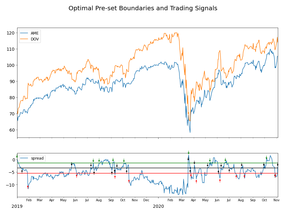
In the remainder of this section, I will demonstrate how to quickly set up a mean-reversion trading strategy based on minimum profit optimization with ArbitrageLab. The assets involved are two S&P 500 stocks, Ametek Inc. (AME), and Dover Corp. (DOV). The price data range from Jan 4th, 2016 to Nov 23th, 2020. The first three years of data were used for boundary optimization and the rest of the data were used for out-of-sample testing.

from arbitragelab.cointegration_approach.minimum_profit import MinimumProfit

# Assume you already have the price of the two stocks stored in a Pandas dataframe "data".
# Initialize the minimum profit optimizer.
optimizer = MinimumProfit(data)

# Split the entire price history into training and trading period.
train_df, trade_df = optimizer.train_test_split(date_cutoff=pd.Timestamp(2019, 1, 1))

# Determine the cointegration coefficient and fit the cointegrated spread with AR(1)
beta_eg, epsilon_t_eg, ar_coeff_eg, ar_resid_eg = optimizer.fit(use_johansen=False, sig_level="95%")

# Optimize the trade boundaries.
optimal_ub, _, _, optimal_mtp, optimal_num_of_trades = optimizer.optimize(ar_coeff_eg, epsilon_t_eg,
                                                                          ar_resid_eg, len(train_df))

# Generate trade signals for both in-sample data and out-of-sample data
trade_signal_is, num_of_shares_is, cond_value_is = optimizer.trade_signal(optimal_ub, optimal_ub,
                                                                          beta_eg, epsilon_t_eg,
                                                                          insample=True)

trade_signal_oos, num_of_shares_oos, cond_value_oos = optimizer.trade_signal(optimal_ub, optimal_ub,
                                                                             beta_eg, epsilon_t_eg,
                                                                             insample=False)

With seven lines of code, a mean-reversion trading strategy has been set up with optimal boundaries. The trade signal generated by this algorithm can be then used for backtesting.

How did the strategy perform? Let’s take a look at in-sample result first.

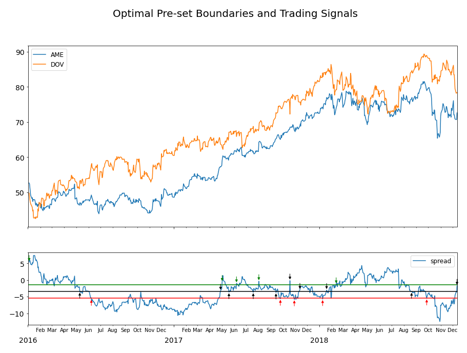
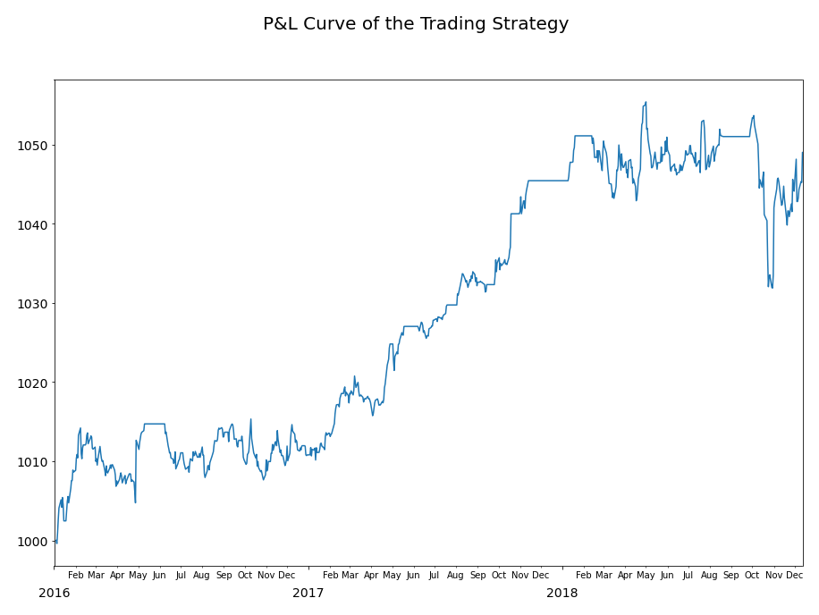
Figure 3. The in-sample performance of the trading strategy based on minimum profit optimization methods. The optimal upper boundary corresponds to the green line in the trading signal chart. The symmetric lower boundary corresponds to the red line in the trading signal chart. The strategy was able to generate a profit in the end of the trading period.

What about out-of-sample performance?

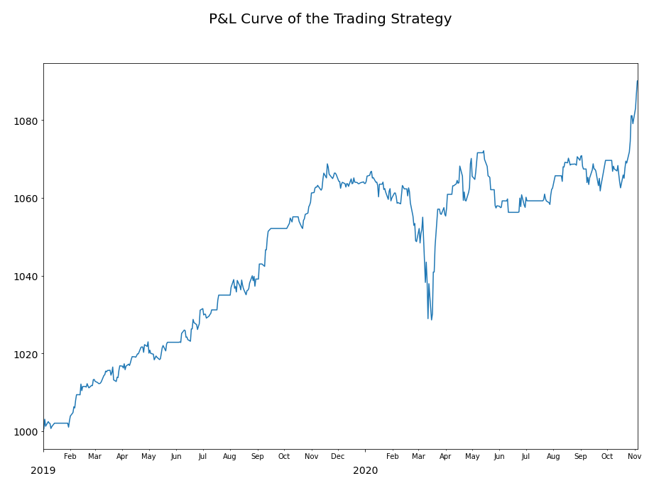
Figure 4. The out-of-sample performance of the trading strategy based on minimum profit optimization methods. The optimal upper boundary corresponds to the green line in the trading signal chart. The symmetric lower boundary corresponds to the red line in the trading signal chart. The strategy was able to generate a profit in the end of the trading period.

The optimal boundary was $2.05$ away from the mean for this cointegrated stock pair, meaning that the minimum profit optimization strategy is able to generate a $\$2.05$ profit trading one unit of the pair. To increase the trade frequency, a symmetric lower boundary at $-2.05$ away from the mean was used for trade initiation as well so that the strategy can both “buy low” and “sell high”. The in-sample results have shown that the average profit per trade is $\$4.90$ , which is higher than the minimum profit per trade $\$2.05$ . The out-of-sample results did not decay significantly, which generated $\$4.74$ per trade on average.

This result was promising as the out-of-sample testing period included the coronavirus market crash, yet the performance was not severely affected. But the minimum profit optimization method is certainly not the holy grail and has its limitations.

We have assumed that the spread follows a stationary AR(1) process. However, the real underlying process of the spread may not be AR(1). As we can see from the trading signal charts, the spread spent a considerable time outside the boundaries. This suggests that the mean first-passage time of an AR(1) process might not yield the best estimates for trade duration and inter-trade intervals. However, a numerical estimation scheme may become unavailable as a result of using a more complicated time series model.

A possible fix to this issue could be try using sliding window instead of cumulative window to optimize the boundary. For example, the minimum profit optimization should be carried out on 6-month rolling price data so that the optimal boundary will not stay fixed throughout the trading period. This may increase the ability of the strategy to adapt to different market regimes.

Conclusions

This article has introduced the minimum profit optimization method on mean-reverting asset pairs and multi-asset portfolios and how it can be used to set up a mean-reversion trading strategy.

Key Takeaways

The optimal boundary can be determined by optimizing trade duration and inter-trade interval.
Trade duration and inter-trade interval can be estimated with mean first-passage time.
If the spread follows a stationary AR(1) process, a numerical algorithm can be applied to estimate trade duration and inter-trade interval in $O(n^3)$ time.
The optimal boundary maximizes the total minimum profit over a trading period.

References

- Basak, G.K. and Ho, K.−W.R. (2004). Level-crossing Probabilities and First-passage Times for Linear Processes. Advance Applied Probability, 36, 643-666.
- Puspaningrum, H., Lin, Y.-X., and Gulati, C. M. (2010). Finding the optimal pre-set boundaries for pairs trading strategy based on cointegration technique. Journal of Statistical Theory and Practice, 4(3):391–419.