Optimal Stopping in Pairs Trading: Ornstein-Uhlenbeck Model
By Valeriia Pervushyna
Join the Reading Group and Community: Stay up to date with the latest developments in Financial Machine Learning!
LEARN MORE ABOUT PAIRS TRADING STRATEGIES WITH “THE DEFINITIVE GUIDE TO PAIRS TRADING”
Introduction
Nothing makes a situation better like good timing. Whether it’s getting a promotion, catching the last train after a night out, meeting the love of your life, or joining a quant community – it is many of small consequential gambles of stopping decisions that get us to that triumphant “Yes!” moment. When outputs may vary, the basic setup of all these problems is the same: we observe some process that involves randomness in it evolving in time. Based only on the knowledge available the person has to decide how to maximize reward or minimize the cost. There is no requirement on how much information has to be available, whether it is scarce or abundant the decision-maker has to make the best choice. Luckily for us, knowing the powers of probability allows us to tilt odds in our favor.
Let’s look at some more mundane problems that can be solved with the little help of optimal-stopping theory.
The first example is the problem of finding a suitable partner, also known as the secretary problem, dowry, or best-choice problem. Imagine, you decide to marry, and to find your perfect other half you conduct an interview with 100 applicants. The decision about an applicant is made immediately. You can not marry candidates who you already rejected, and if you are not married after interviewing candidate 99 – you have to marry candidate 100. Of course, you can choose the first applicant and get a 1% chance of getting the best spouse. But there is a way to marry the absolute best candidate more than one-third of the time.
The rule is to reject ![]() potential spouses, and then choose the first applicant who is better than every applicant interviewed so far.
potential spouses, and then choose the first applicant who is better than every applicant interviewed so far.
The various problems similar to the ‘secretary problem’ create so-called ‘search theory’, that has especially focused on a worker’s search for the highest-paying job or a consumer’s search for the best deal on wanted goods.
Optimal stopping is also encountered in house selling. For example, if you wish to sell a house. Each day you are offered ![]() for your house, and pay
for your house, and pay ![]() to continue advertising it. If you sell your house on day
to continue advertising it. If you sell your house on day ![]() , you will earn
, you will earn ![]() , where
, where ![]() . You maximize the amount you earn by choosing the best stopping rule.
. You maximize the amount you earn by choosing the best stopping rule.
The field of optimal stopping problems is broad and vast, it ranges from option pricing with the Black-Scholes model to choosing the best parking spot when going to buy groceries. But what if I tell you that there is a simple and elegant way to use it for the statistical arbitrage?
Welcome to Part 1 of the series of blog posts on optimal stopping problems for statistical arbitrage. And today we are going to talk about the Ornstein-Uhlenbeck model application to optimal stopping problems in pairs trading.
Mean-reversion
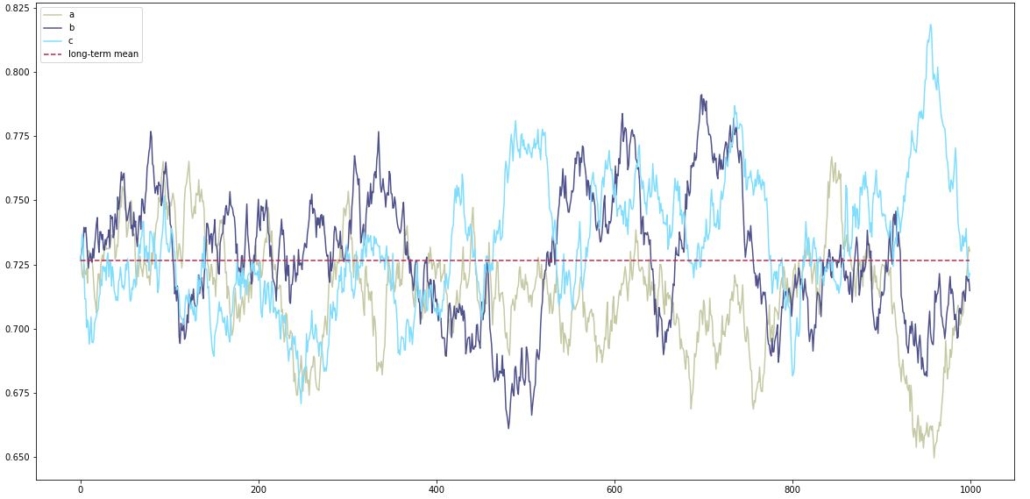
Mean-reverting processes and their long-term mean.
But before that, we need to start with something that will allow the statistical arbitrage in the first place – mean-reversion.
Mean-reversion is a financial term for the assumption that a stock’s price will tend to return to the average price over time. Some asset prices are naturally mean-reverted: commodities, foreign exchange rates, volatility indices, equities – all of those can be modeled with mean-reverting processes, alongside with interest rate and default risk.
However, there is a much more lucrative approach that also allows for greater freedom of choice for the investor – pairs-trading. Facilitated by many hedge-fund managers, creation of the mean-reverting portfolios gave the ability to both pick almost any asset you’d want to trade and simultaneously rely on rigid mathematical concepts in the decision-making process. The only requirement to be is that the pair chosen has to be correlated or co-moving. Technically speaking, a portfolio is created by longing an ![]() amount of one asset
amount of one asset ![]() and shorting
and shorting ![]() amount of a second asset
amount of a second asset ![]() .
.
\begin{aligned}X_t^{\alpha,\beta} = \alpha S^{(1)} – \beta S^{(2)}, t \geq 0\end{aligned}
It is no surprise that such spreads are widely used for statistical arbitrage.
Looking deeper, one very important commonly faced problem still stands – how to determine when to open and close the position. Should an investor wait or close the position immediately? When is it the optimal time to enter the market? All these questions bring us to a brilliant idea: what if we could look at it as an optimal stopping problem? Can we create a procedure that will give us the means to predict the best time to enter or liquidate the position?
For an answer to this question, we turn to a book by Professor Tim Leung and Xin Li: “Optimal Mean reversion Trading: Mathematical Analysis and Practical Applications“. We will showcase how the widely known Ornstein-Uhlenbeck process can be used to create your optimal mean-reverted portfolio and to also find the solution for the optimal timing of trades problem.
The work of Professor Tim Leung
Ornstein-Uhlenbeck model is established by the following SDE:
\begin{aligned}dX_t = \mu(\theta – X_t)dt + \sigma dB_t,\end{aligned}
\begin{aligned}\mu, \sigma > 0,\end{aligned}
\begin{aligned}\theta \in \mathbb{R},\end{aligned}
\begin{aligned}B\ -\text{a standard Brownian motion}\end{aligned}
Where:
![]() − long term mean level, all future trajectories of
− long term mean level, all future trajectories of ![]() will evolve around a mean level
will evolve around a mean level ![]() in the long run.
in the long run.
![]() – the speed of reversion, characterizes the velocity at which such trajectories will regroup around
– the speed of reversion, characterizes the velocity at which such trajectories will regroup around ![]()
in time.
![]() – instantaneous volatility, measures instant by instant the amplitude of randomness entering the system. Higher values imply more randomness.
– instantaneous volatility, measures instant by instant the amplitude of randomness entering the system. Higher values imply more randomness.
Note that we are using the same notation as used in the book, so the meaning behind theta and mu parameter may differ from other sources (Wikipedia, etc.).
To create an optimal portfolio using this model we can without the loss of generality presume that ![]() while varying
while varying ![]() , since our main goal during this step can be simplified to finding an optimal ratio between the assets.
, since our main goal during this step can be simplified to finding an optimal ratio between the assets.
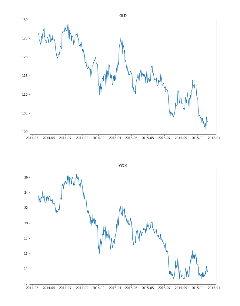
Exemplary co-moving assets.
We observe the resulting portfolio values for every strategy ![]() realized over an
realized over an ![]() -day period. To fit the model to our data and find optimal parameters we define the average log-likelihood function. Our log-likelihood function is dependent on our
-day period. To fit the model to our data and find optimal parameters we define the average log-likelihood function. Our log-likelihood function is dependent on our ![]() coefficient and the OU model’s parameters theta, mu, and sigma.
coefficient and the OU model’s parameters theta, mu, and sigma.
Maximizing the log-likelihood function by applying maximum likelihood estimation(MLE) we can determine the parameters of the model and fit the observed portfolio prices to an OU process. Let’s denote the maximized average log-likelihood by ![]() . Then for every
. Then for every ![]() , we choose
, we choose ![]() , where:
, where:
\begin{aligned} \beta^* = \underset{\beta}{\arg\max}\ \hat{\ell}(\theta^*,\mu^*,\sigma^*|x_0^{\alpha\beta},x_1^{\alpha\beta},\cdots,x_n^{\alpha\beta}) \end{aligned}
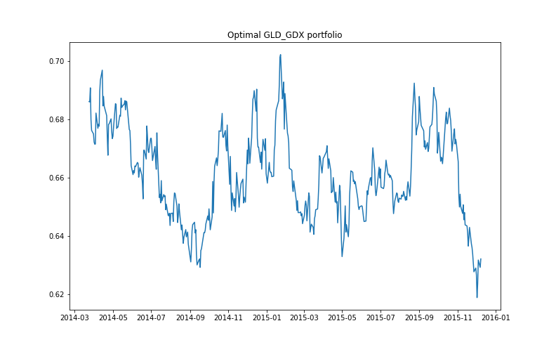
To create the most fitting to an OU-model portfolio, hence optimal and more mean-reverted one.
Optimal mean-reverting portfolio constructed by maximizing the log-likelihood function.
The next step is to establish our optimal stopping problem: suppose the investor already has a position with a value process ![]() that follows the OU process. When the investor closes his position at the time
that follows the OU process. When the investor closes his position at the time ![]() he receives the value
he receives the value ![]() and pays a constant transaction cost
and pays a constant transaction cost ![]() . To maximize the expected discounted value we need to solve the optimal stopping problem:
. To maximize the expected discounted value we need to solve the optimal stopping problem:
\begin{aligned} V(x) = \underset{\tau \in T}{\sup} \mathbb{E}_x{e^{-r \tau} ((X_{\tau} – c_s)| X_0 = x)} \end{aligned}
where ![]() denotes the set of all possible stopping times and
denotes the set of all possible stopping times and ![]() is our subjective constant discount rate and
is our subjective constant discount rate and ![]() represents the expected liquidation value accounted with
represents the expected liquidation value accounted with ![]() .
.
The next logical step is to formalize the optimal entry problem since the future optimal value of liquidation minus current price and transaction cost constitute the cost of entering the trade:
\begin{aligned} J(x) = \underset{\nu \in T}{\sup} \mathbb{E}_x{e^{-\hat{r} \tau} ((V(X_{\nu}) – X_{\nu} – c_b)| X_0 = x)} \end{aligned}
Sometimes an investor would like to include a stop-loss level. If the price of a portfolio will ever reach this level, then the position will be closed immediately. So the problem is reformulated in the following way:
\begin{aligned} V(x)_L = \underset{\tau \in T}{\sup} \mathbb{E}_x{e^{-r \tau \wedge \tau_L} ((X_{\tau \wedge \tau_L} – c_s)| X_0 = x)} \end{aligned}
\begin{aligned} J(x)_L = \underset{\nu \in T}{\sup} \mathbb{E}_x{e^{-\hat{r} \tau} ((V_L(X_{\nu}) – X_{\nu} – c_b)| X_0 = x)} \end{aligned}
The analytical solutions for the optimal stopping problems are presented and proven in Optimal Mean reversion Trading: Mathematical Analysis and Practical Applications by Professor Tim Leung and Xin Li.
Our goal is to find the single best entry/liquidation value pair to get the biggest amount of profit from one trade.
However similar both formulations may look, the results we get are slightly different.
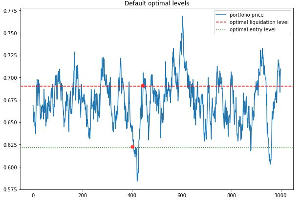
Example of Optimal Entry and Exit for a Mean-Reverting Processes
In the default formulation as a result we are getting two values – optimal entry level ![]() and optimal liquidation level
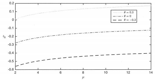
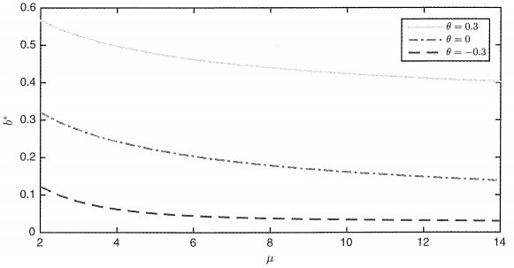
and optimal liquidation level ![]() . Since the obtained values are dependent on the OU model parameters we can observe further correlations:
. Since the obtained values are dependent on the OU model parameters we can observe further correlations:
The optimal entry-level d* vs speed of mean reversion (Professor Tim Leung and Xin Li, 2015).
The optimal liquidation level b* vs speed of mean reversion (Professor Tim Leung and Xin Li, 2015).
- With the increase of the long-term mean both entry and liquidation value tend to be higher.
- Faster mean reversion means closer buy and sell levels (where the sell-level value is going to decrease and the entry value – increase.
- The increase in volatility sets the buy and set levels further apart. So if the volatility is high it is possible to delay both entry and exit levels to seek a wider spread.
- High transaction costs also usually mean higher sell levels since we wish to compensate for the loss on transaction costs.
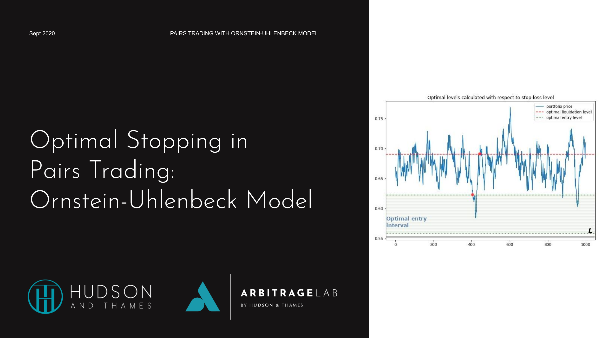
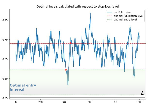
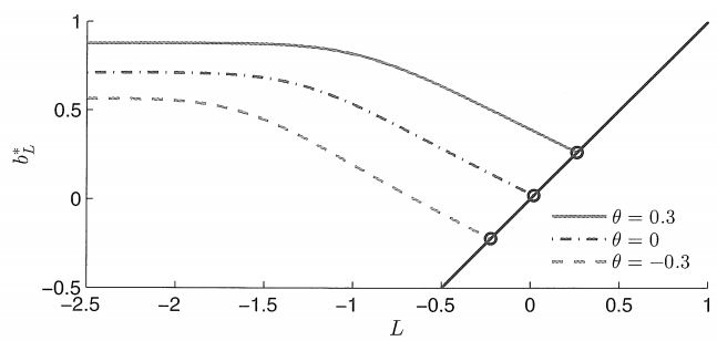
In the case of the problem with the addition of the stop-loss:
The optimal exit threshold vs stop-loss level. The straight line lies where ![]() . (Professor Tim Leung and Xin Li, 2015).
. (Professor Tim Leung and Xin Li, 2015).
- All correlations from the default model still hold true.
- The optimal liquidation level is strictly decreasing with the increase of the stop-loss level.
- The optimal entry-level becomes an optimal entry interval set strictly above the stop-loss level (L). The signal for buying, in this case, is when the price of a portfolio reaches one of the interval bounds. Particular case being if the current price is between the lower bound and a stop-loss level it is still optimal to wait to avoid exiting at a loss.
“Our model can be considered as the building block for the problem with any finite number of sequential trades” – Professor Tim Leung and Xin Li, 2015.
Conclusion
We encounter myriads of small optimal stopping problems during our lifetime. Asking for a raise, getting a better deal on your car, or picking the best parking spot – they exist in all the areas of life that require decision-making to maximize the good or minimize the bad. Luckily, with a help of stochastic calculus and optimal stopping theory, we can quantify our decision-making process and get the strategy that will give us the best result possible with the most probability. It is only natural that people would try to use it in a world where knowing where to stop is so crucial – quantitative finance
Following the work of Professor Tim Leung and Xin Lee, we explored how the Ornstein-Uhlenbeck process known for modelling mean-reverting interest rates, currency exchange rates, and commodity prices can be used in pairs trading and statistical arbitrage. The two-step process looks the following way: first, we fit the OU process to our pairs-trading portfolio and also choose the optimal ratio between two assets by maximizing the average log-likelihood function, achieving the best mean-reversion and the best fit at the same time. The second step is setting the optimal stopping problem and subsequently solving it. We maximize our expected discounted values of entry and liquidation to find the optimal levels at which we buy or sell our spread. It is also possible to expand the problem by adding the stop-loss level. Both solutions are found with the presumption of the single entry and exit point.
We will talk about the expansion of the optimal stopping problem – the optimal switching problem that accounts for multiple possible entry and exit points in the next blog post on XOU model.
Check out our lecture on the topic:
References
- Leung, Tim, and Xin Li. “Optimal Mean Reversion Trading: Mathematical Analysis and Practical Applications.” World Scientific Publishing Company (2015).

