Optimal Trading Thresholds for the O-U Process
by Andy Lin and Illya Barziy
Join the Reading Group and Community: Stay up to date with the latest developments in Financial Machine Learning!
Introduction
Pairs trading or statistical arbitrage is a famous strategy among institutional and individual investors since the 1990s. The concept behind this kind of strategy is straightforward. If the prices of assets move together historically, this tendency is likely to continue in the future. When the spread of the prices diverges from its long-term mean, one can short sell the over-priced stock, buy the under-priced one, and wait for the spread to converge to take the profit.
In general, to develop a pairs trading strategy, we need to solve two major issues, the first is how to select assets to form a process with mean reversion properties, and the second is how to decide when to trade. A standard answer to the second question is to enter the market when the tradable spread process deviates from its long-term mean by a fixed amount. For example, N times (usually, 2-3) the historical standard deviation of the tradable process is a common threshold used in practice. As for how to determine the N, one of the used approaches is to solve the optimization problem based on historical asset prices, maximizing the total return of the strategy or its Sharpe ratio.
The papers that are covered in this article propose a different way to determine the entry and exit thresholds for a pairs trading strategy. Instead of maximizing strategy performance with historical data, the approach provided by the reference papers calculates the optimal trading thresholds by theoretically optimizing the expected returns per unit of time. This approach was first discussed in Bertram, W. K. (2010) and extended by Zeng, Z. and Lee, C.-G. (2014).
Basics
In Bertram, W. K. (2010), the author derives analytic formulae for statistical arbitrage trading where the price of an asset follows an exponential Ornstein-Uhlenbeck process. By framing the problem in terms of the first-passage time of the process, he first derives the expressions for the mean and the variance of the trade length. Then he derives the formulae for the expected return and the variance of the return per unit of time. Finally, a solution to the problem of choosing optimal trading thresholds is proposed by maximizing the expected return and the Sharpe ratio.
Below we will first describe the assumptions and term definitions used in this theoretical approach, then introduce the formulas derived by the author, and finally, explain how the optimal trading strategies work. It is worth noting that the paper assumes that the long-term mean of the O-U process is zero, however, we have extended the model so that the O-U process with a non-zero mean can also be used in this method. We use to denote the long-term mean, for mean-reversion speed, and for the amplitude of randomness of the O-U process, which is different from the reference paper. This is done to be consistent with our previous articles that are using a concept of the Ornstein-Uhlenbeck process with these parameter names.
Assumptions
Price of the Traded Security
The model defines the price of the traded security ![]() as,
as,
![]()
where ![]() follows an O-U process and satisfies the following stochastic differential equation,
follows an O-U process and satisfies the following stochastic differential equation,
![]()
where ![]() is the long-term mean,
is the long-term mean, ![]() is speed at which the values will regroup around the long-term mean and
is speed at which the values will regroup around the long-term mean and ![]() is the amplitude of randomness of the O-U process.
is the amplitude of randomness of the O-U process.
Trading Strategy
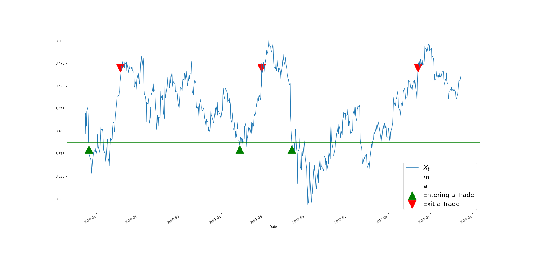
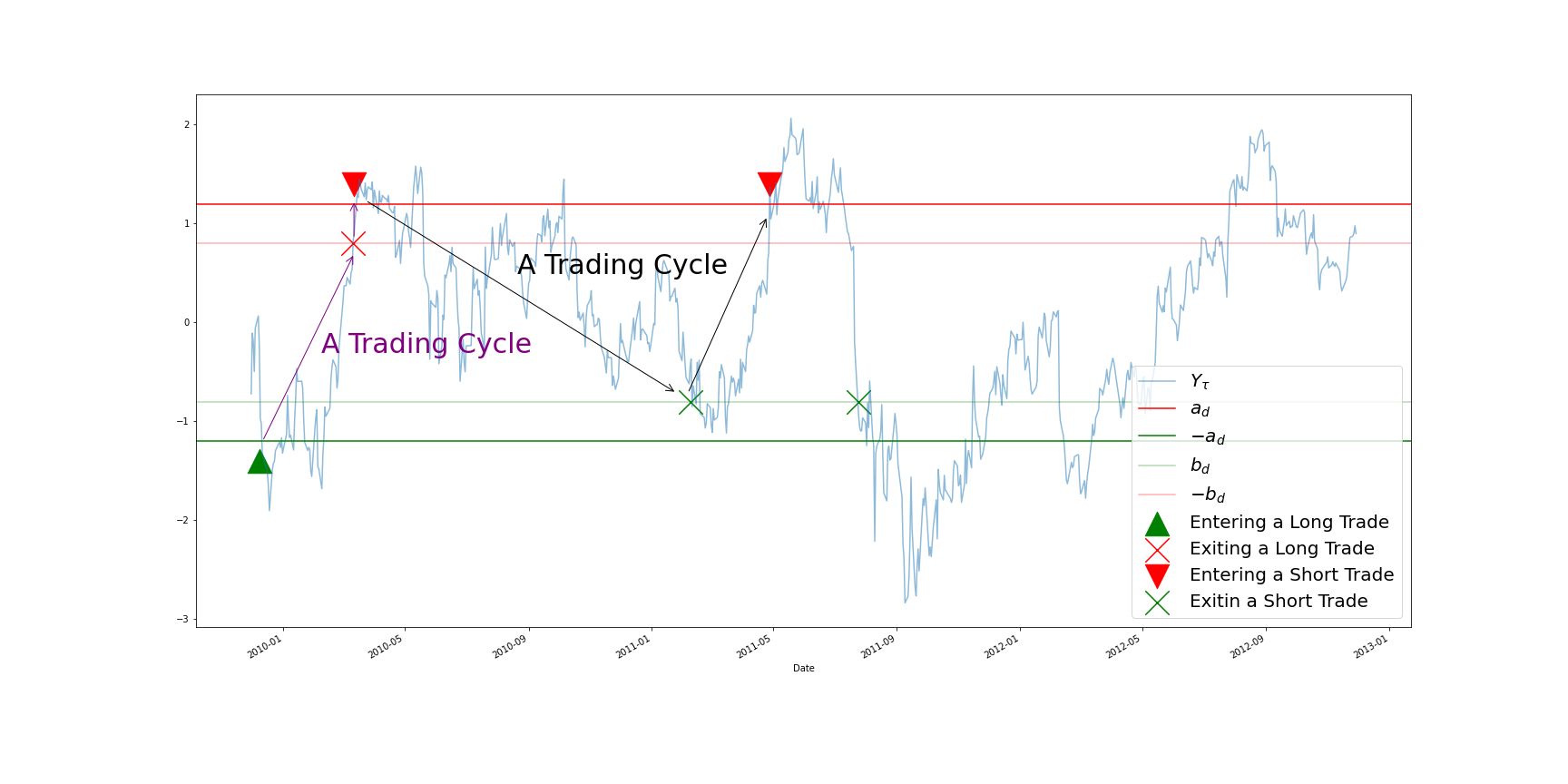
The trading strategy is defined as an act of entering a trade when ![]() , exiting the trade at
, exiting the trade at ![]() , where
, where ![]() . The paper here assumes that traders can only make a long trade on the traded security. The original model was adjusted and this assumption was later removed in the work of Zeng, Z. and Lee, C.-G. (2014) to obtain a more versatile trading model.
. The paper here assumes that traders can only make a long trade on the traded security. The original model was adjusted and this assumption was later removed in the work of Zeng, Z. and Lee, C.-G. (2014) to obtain a more versatile trading model.
Trading Cycle
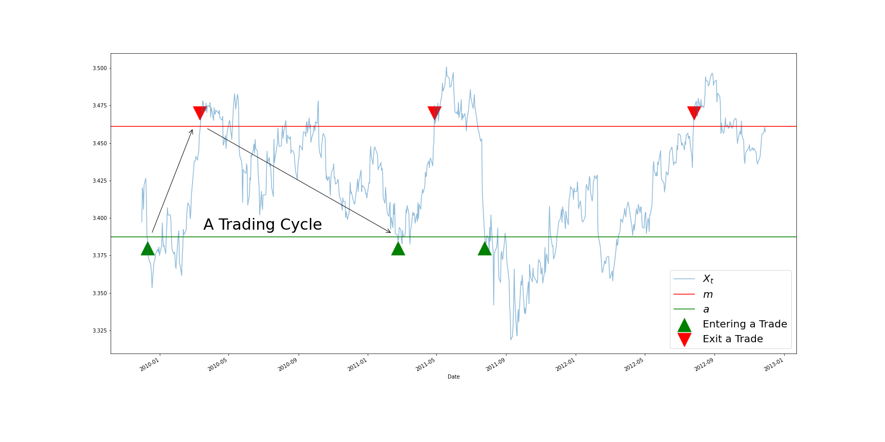
The trading cycle is completed as ![]() change from
change from ![]() to
to ![]() , then back to
, then back to ![]() .
.
Trade Length
The trade length T is defined as the time needed to complete a trading cycle.
Analytic Formulae
Here we simply show the results provided by the paper. One can see the reference paper for the detailed derivation process.
Mean and Variance of the Trade Length
![]()
where ![]() is the imaginary error function.
is the imaginary error function.
![]()
where
![]()
![]()
where ![]() and
and ![]() is the digamma function.
is the digamma function.
Mean and Variance of the Trading Strategy Return per Unit of Time
![]()
![]()
where ![]() gives the continuously compound rate of return for a single trade and accounting for the transaction cost.
gives the continuously compound rate of return for a single trade and accounting for the transaction cost.
Optimal Strategies
To calculate an optimal trading strategy, we seek to choose optimal entry and exit thresholds that maximize the expected return or the Sharpe ratio (depending on our goal) per unit of time for a given transaction cost/risk-free rate.
Get Optimal Thresholds by Maximizing the Expected Return / Sharpe Ratio
This paper shows that the maximum expected return/Sharpe ratio occurs when ![]() . Since we have assumed that
. Since we have assumed that ![]() , this implies that
, this implies that ![]() . Therefore, for a given transaction cost/risk-free rate, the following equation can be maximized to find optimal
. Therefore, for a given transaction cost/risk-free rate, the following equation can be maximized to find optimal ![]() and
and ![]() .
.
![]()
![]()
where ![]() and
and ![]() is the risk-free rate.
is the risk-free rate.
Extension
In Zeng, Z. and Lee, C.-G. (2014), the authors enhance the work of Bertram, W. K. (2010), which only allows long positions on a tradable process when finding the optimal trading thresholds. To also allow short positions, the authors of the first paper derive a polynomial expression for the expectation of the first-passage time of an O-U process with a two-sided boundary. Then they simplify the problem of optimizing the expected return per unit of time to a problem of solving an equation.
Below we will first describe the assumptions and term definitions of the extended approach, then introduce the formulas derived by the authors, explain the optimal trading strategies, and finally, replicate a trading example provided in the paper. We’d like to note that the paper didn’t give the formula of ![]() , we derived it ourselves to ensure the module’s integrity. We use
, we derived it ourselves to ensure the module’s integrity. We use ![]() to denote the long-term mean,
to denote the long-term mean, ![]() for mean-reversion speed, and
for mean-reversion speed, and ![]() for the amplitude of randomness of the O-U process, which is, again, different from the parameter naming in the reference paper.
for the amplitude of randomness of the O-U process, which is, again, different from the parameter naming in the reference paper.
Assumptions
Price of the Traded Security
The model defines the price of the traded security ![]() as,
as,
![]()
where ![]() follows an O-U process and satisfies the following stochastic differential equation,
follows an O-U process and satisfies the following stochastic differential equation,
![]()
where ![]() is the long-term mean,
is the long-term mean, ![]() is the speed at which the values will regroup around the long-term mean and
is the speed at which the values will regroup around the long-term mean and ![]() is the amplitude of randomness of the O-U process.
is the amplitude of randomness of the O-U process.
Trading Strategy
The Trading strategy is defined as follows:
![]()
where ![]() ,
, ![]() is the entry and exit thresholds in the dimensionless system, respectively. The
is the entry and exit thresholds in the dimensionless system, respectively. The ![]() is a dimensionless series transformed from the original time series
is a dimensionless series transformed from the original time series ![]() using the following formula:
using the following formula:

Trading Cycle
The trading cycle is completed as ![]() change from
change from ![]() to
to ![]() , then back to
, then back to ![]() or
or ![]() .
.
Trade Length
The trade length ![]() is defined as the time needed to complete a trading cycle.
is defined as the time needed to complete a trading cycle.
Analytic Formulae
Mean and Variance of the Trade Length
![]()
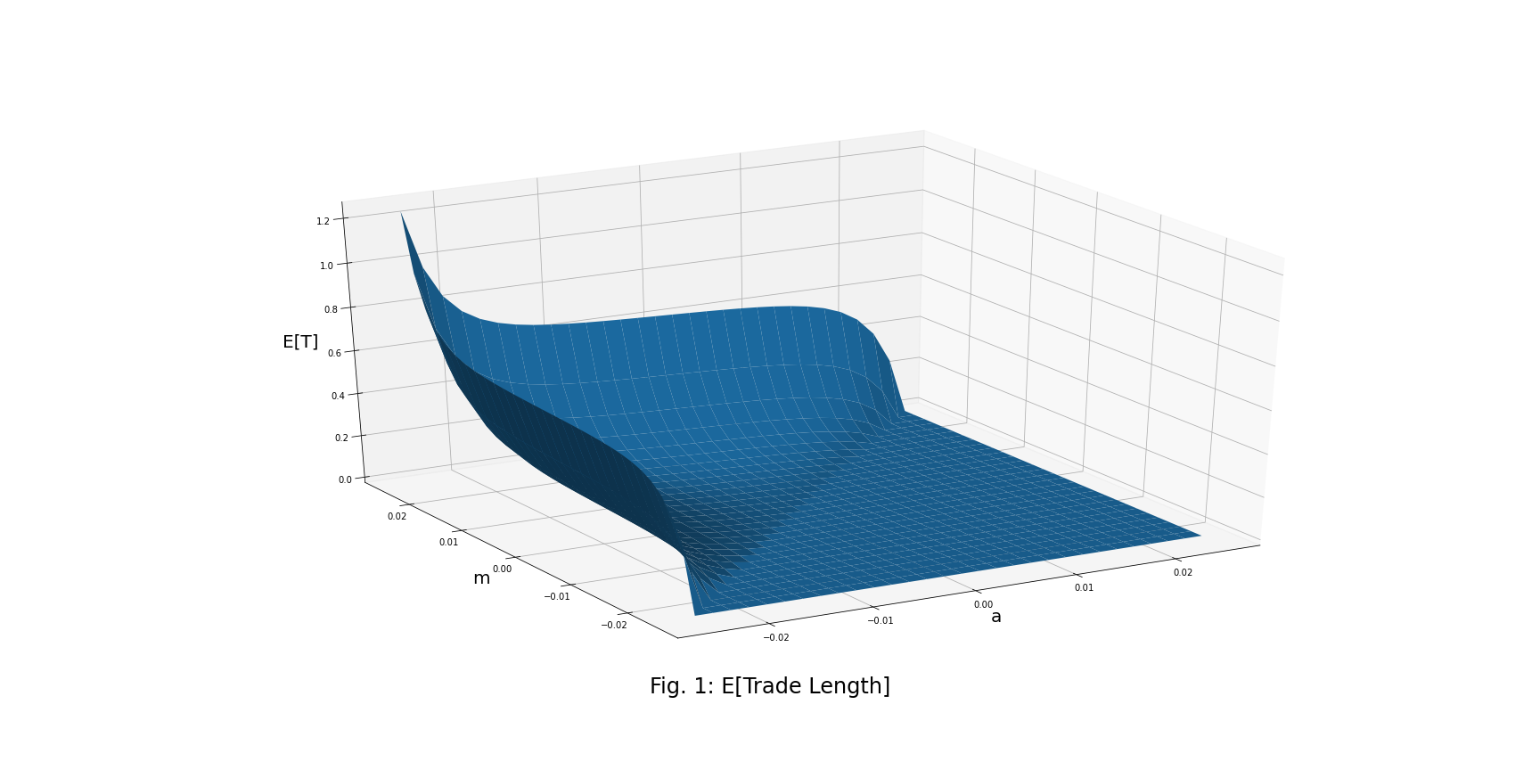
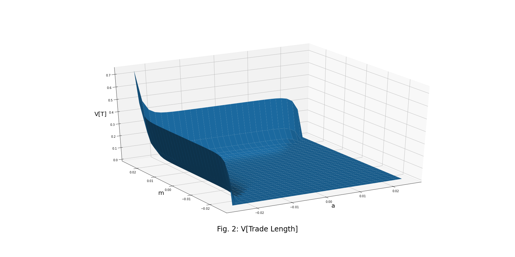
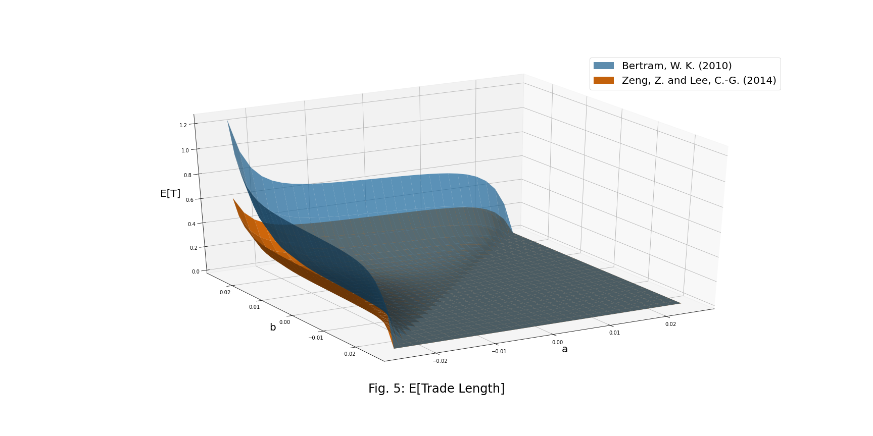
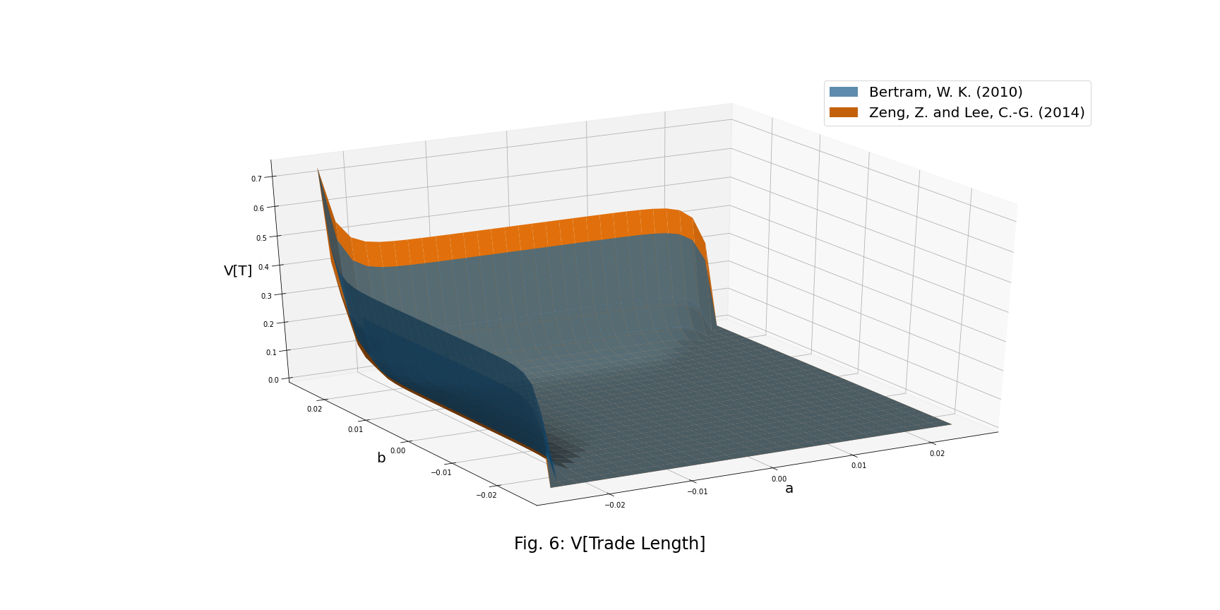
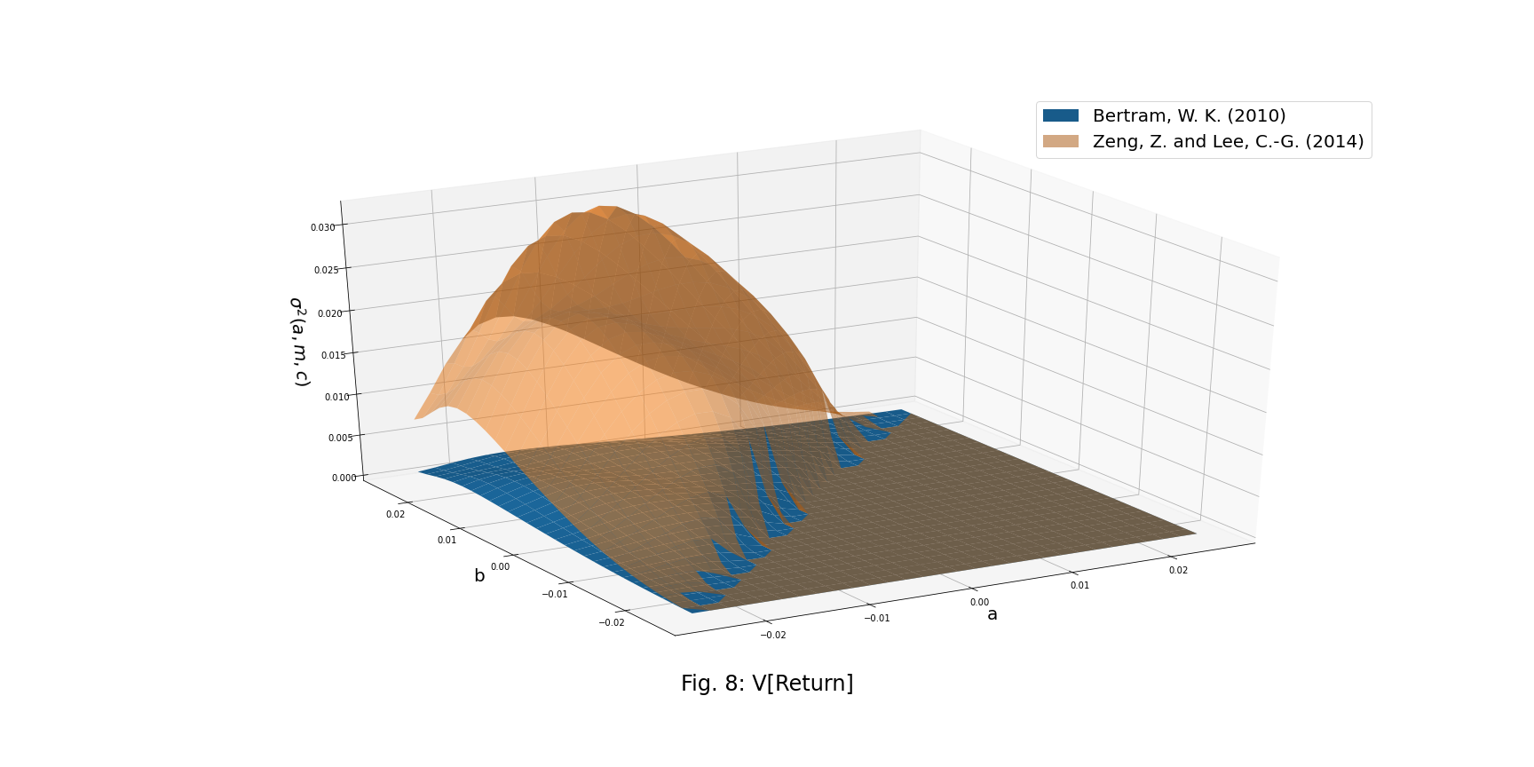
The figure below shows that since we calculate the expected time of the first-passage of an O-U process with a two-sided boundary, we will get a minor E[T] under the same O-U process parameters, in comparison to E[T] from the original paper.
![]()
where ![]() is the variance of the time taken for the O-U process to travel from
is the variance of the time taken for the O-U process to travel from ![]() to
to ![]() , and
, and ![]() is the variance of the time taken for the O-U process to travel from
is the variance of the time taken for the O-U process to travel from ![]() to
to ![]() or
or ![]() .
.
![]()
where
![]()
![]()
![]()
where
![]()
![]()
where
![]()
![]()
where
![]()
where
![]()
Mean and Variance of the Trading Strategy Return per Unit of Time
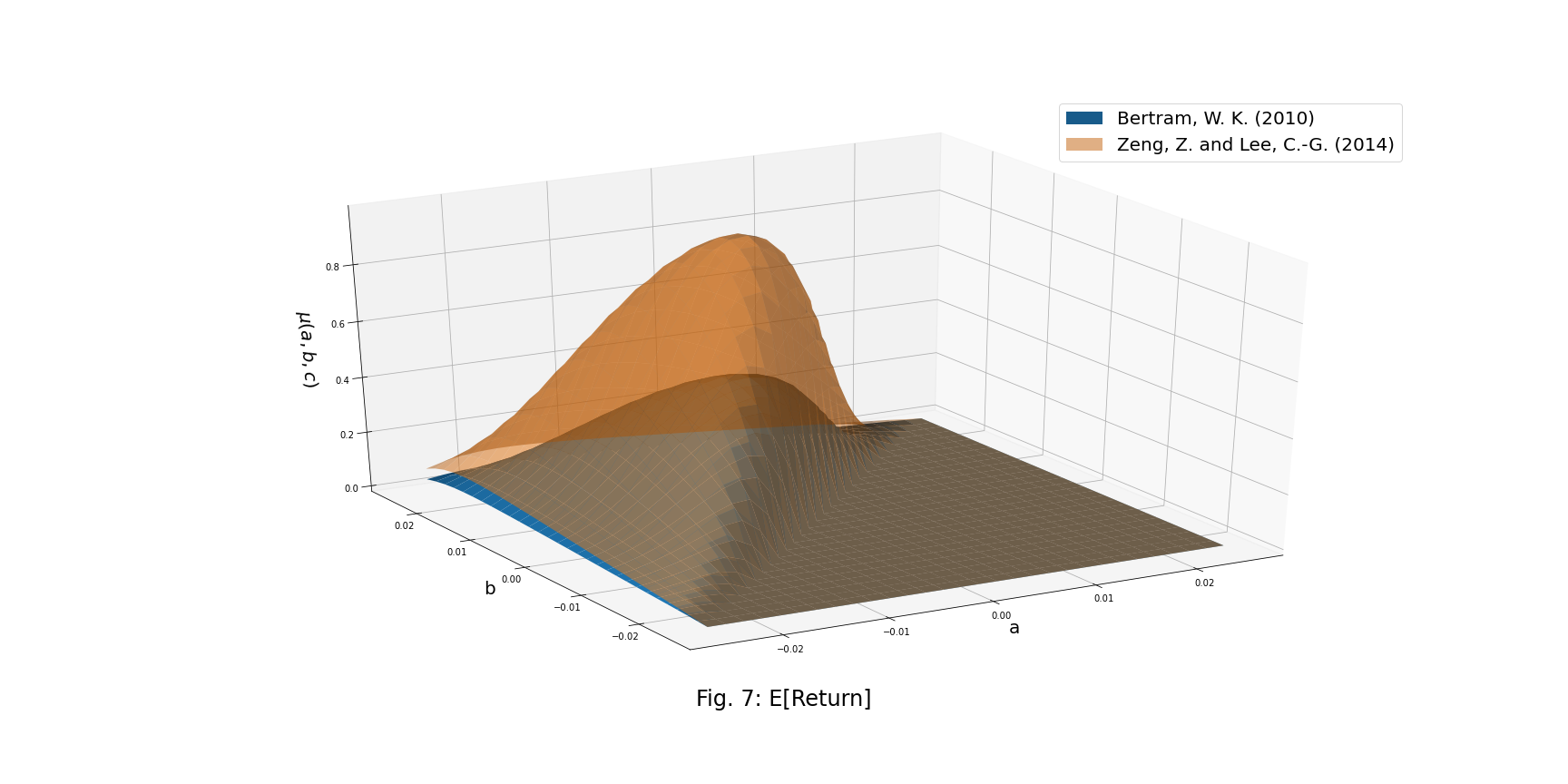
![]()
![]()
where ![]() gives the continuously compound rate of return for a single trade and accounting for the transaction cost.
gives the continuously compound rate of return for a single trade and accounting for the transaction cost.
Optimal Strategies
To calculate an optimal trading strategy, we seek to choose optimal entry and exit thresholds that maximize the expected return per unit of time for a given transaction cost.
Get Optimal Thresholds by Maximizing the Expected Return
Conventional Optimal Rule
When ![]() , this paper shows that the maximum expected return occurs when
, this paper shows that the maximum expected return occurs when ![]() . Therefore, for a given transaction cost, the following equation can be solved to find optimal
. Therefore, for a given transaction cost, the following equation can be solved to find optimal ![]() .
.
![]()
![]()
New Optimal Rule
When ![]() , this paper shows that the maximum expected return occurs when
, this paper shows that the maximum expected return occurs when ![]() . Therefore, for a given transaction cost, the following equation can be solved to find optimal
. Therefore, for a given transaction cost, the following equation can be solved to find optimal ![]() .
.
![]()
![]()
Back Transform from the Dimensionless System
After calculating optimal thresholds in the dimensionless system, we need to use the following formula to transform them back to the original system.
![]()
where
![]()
where ![]() ,
, ![]() denotes the entry and exit thresholds for a short position,
denotes the entry and exit thresholds for a short position, ![]() ,
, ![]() denotes the entry and exit thresholds for a long position.
denotes the entry and exit thresholds for a long position.
Trading Example
This trading example is replicated from the reference paper.
Backtesting Parameters
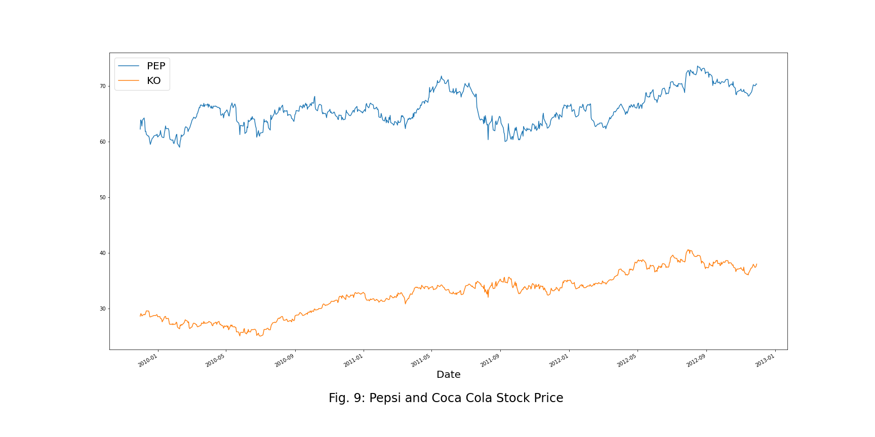
- Pair: Pepsi and Coca Cola
- Spread Series:

- O-U Process parameters:
 ,
,  and
and 
Trading Thresholds
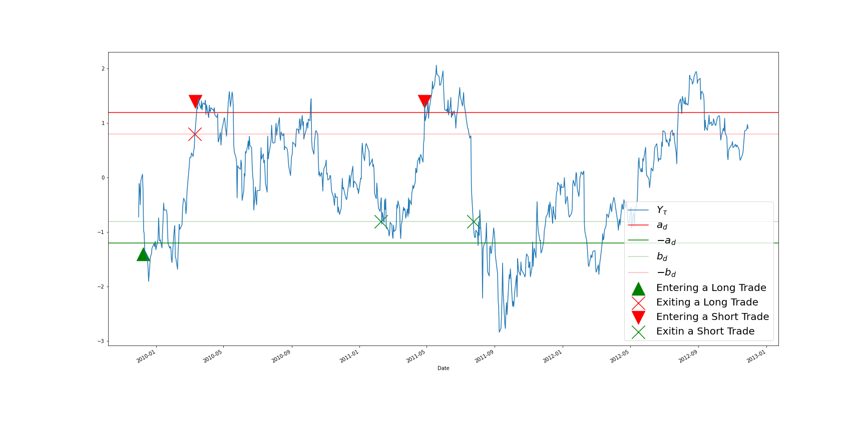
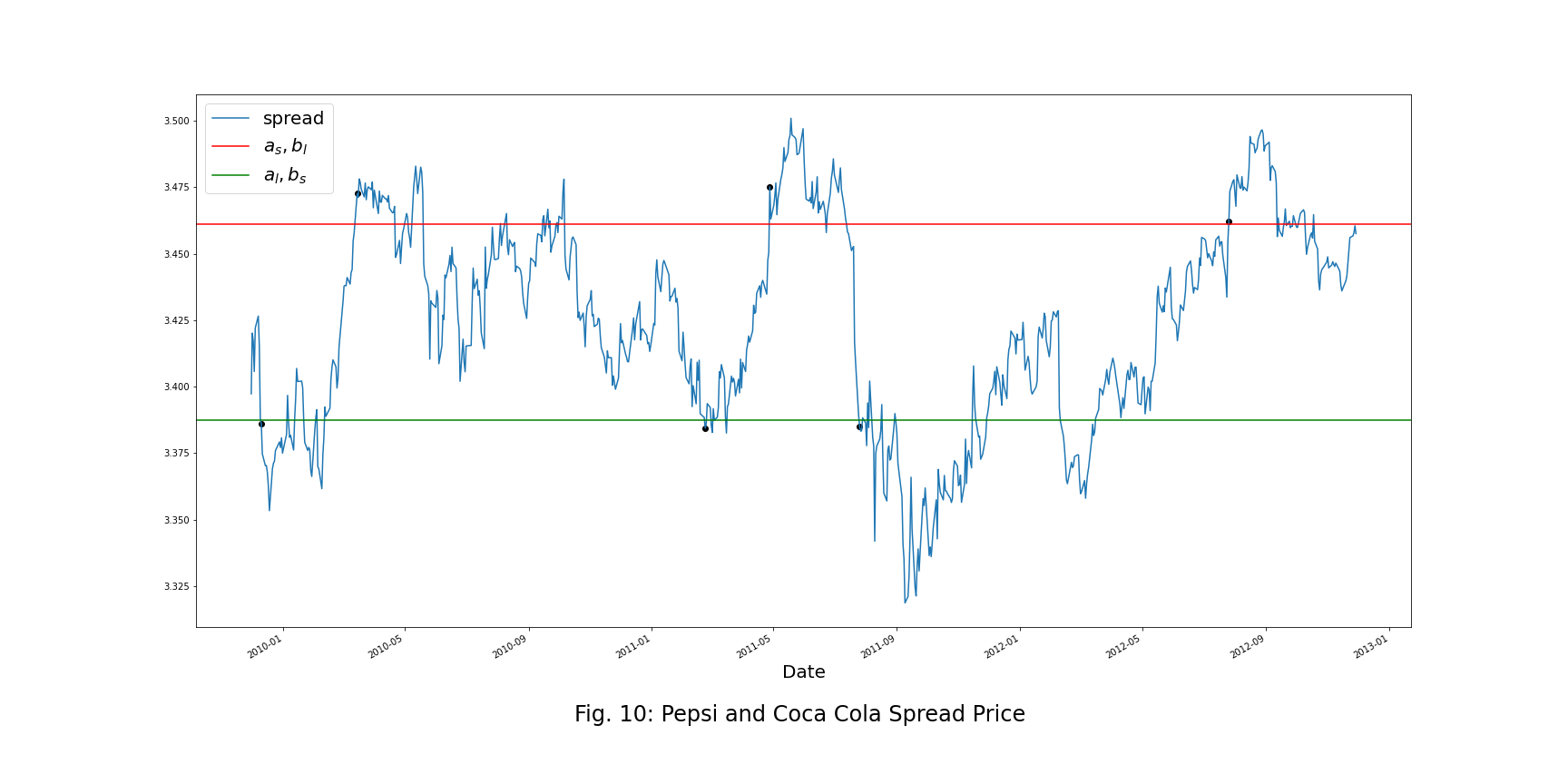
By setting the transaction costs = 0.02 and using the new optimal rule, we can get the trading thresholds as below:
![]()
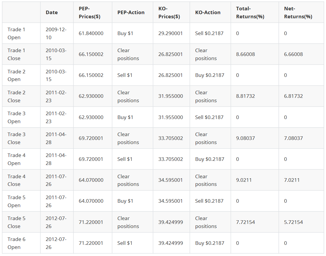
The following table shows the detailed status of each transaction.
Strategy Example
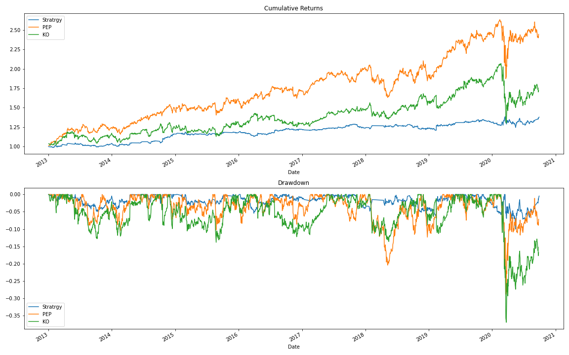
Here we provide a complete pairs trading strategy extend from the trading example above.
Backtesting Parameters
- Pair: Pepsi and Coca Cola
- Spread Series: If we assume the training period for fitting the O-U process is from
 to
to  , and the testing period is from
  to
to  , then
![]()
- O-U Process parameters:
 ,
,  and
and  are determined by fitting the O-U process to the training data.
  ,
,  ,
,  and
and  are redetermined every 6-months with a 1-year history. The fitting method used can be found on pp. 12-13 of the following book: Tim Leung and Xin Li, Optimal Mean reversion Trading: Mathematical Analysis and Practical Applications. The optimal trading strategy from this book was described in one of our previous articles, which can be found here.
Trading Thresholds
By setting the transaction costs = 0.004 per round trip for the pair and using the conventional optimal rule, we can calculate the optimal trading thresholds and conclude the backtesting on the testing dataset.
Performance
From the table below, we can see that the strategy’s returns are lower than the returns from just Buy & Hold of either of the stocks in a pair. However, the risks of such a strategy are significantly lower than the risks of Buy & Hold, which might pose more interest for more risk-averse traders.
Conclusion
The papers covered in this article provide analytic formulas to calculate the trade length’s mean and variance when trading on the O-U process. These allow us to calculate the expected return and the variance per unit of time of the strategy. Therefore, we can reduce the optimal trading thresholds finding problem to a simple maximization problem. In Zeng, Z. and Lee, C.-G. (2014), the authors also provided an empirical trading example to showcase that the theoretical approach works in practice and we were able to replicate the results on a new dataset. Confirming that the described strategy can be used on newer data.
At the end of this article, we provide the details of the performed backtesting of the optimal thresholds strategy. Although the strategy looks complete, there are still some details that can be improved or further studied:
- Stop-loss policy.
-
- It is essential to have a stop-loss policy for a pairs trading strategy. If the assets in a pair encounter structural breaks, the spread may never diverge, and the investor might have an unacceptable loss if no stop-loss rule is added.
- An idea that came to our minds when working with the reference papers. A good point for setting a stop-loss may be a time when the actual trade length exceeds the expected trade length plus N times the historical standard deviation of the trade length.
- Whether the O-U process is fitting good to a tradable process.
-
- When using real-world data, we often encounter problems related to the O-U process not being well fitted or cannot be fitted to a given dataset. A set of actions to complete if a good fit to the O-U process is not found may be a good topic for further exploration.
References
- Bertram, W. K., 2010. Analytic solutions for optimal statistical arbitrage trading. Physica A: Statistical Mechanics and its Applications, 389(11): 2234–2243.
- Zeng, Z. and Lee, C.-G., 2014. Pairs trading: optimal thresholds and profitability. Quantitative Finance, 14(11): 1881–1893.
- Ricciardi, L. and Sato, S., 1988. First-passage-time density and moments of the Ornstein–Uhlenbeck process. Journal of Applied Probability, 25(1): 43–57.

