Pairs Trading Based on Renko and Kagi Models

by Andy Lin and Illya Barziy

Join the Reading Group and Community: Stay up to date with the latest developments in Financial Machine Learning!

Introduction

A group of strategies, named statistical arbitrage or pairs trading strategies are well-known for being market-neutral gained their popularity among institutional and individual investors. In general, to develop a pairs trading strategy, one needs to figure out two aspects, the first is how to select assets to form a process with mean-reverting properties, and the second is how to decide when and how to trade such process. In recent years, many methods have been proposed to answer these two questions. Fitting the spread to an O-U process, cointegration tests, and stochastic control methods are commonly used but are theoretically complicated. For the most part, the trading strategies constructed using these approaches aim to exploit the mean-reverting nature of the constructed spread.

The work by Bogomolov T. (2013) proposes a novel approach to pairs trading based on the idea of Renko and Kagi charts. This approach exploits statistical information about the variability of the tradable process. There is no need for complicated mathematical derivations, and no strict assumptions have to be made regarding the spread price properties. The trading strategy based on Renko and Kagi models is built on defining how far the process should move in one direction from the turning point before trading in the opposite direction becomes potentially profitable by measuring the variability of the process.

This is the third article in a series dedicated to Time Series Approach Pairs Trading Strategies. If you’ve missed previous ones, we are attaching links to them below:

Basic Concepts

The key idea of this approach is first to determine the turning points and their confirmation points of the tradable process. Then the set of characteristics and statistics of the turning points is defined to determine which trading strategy and pair selection method to use for a chosen asset pair. Although the following descriptions and properties are defined under the assumption that the tradable process is continuous, the concepts are also applicable to discrete processes, like real-world data on asset prices. One can study the reference paper for more detailed discussions on this topic.

H-Construction

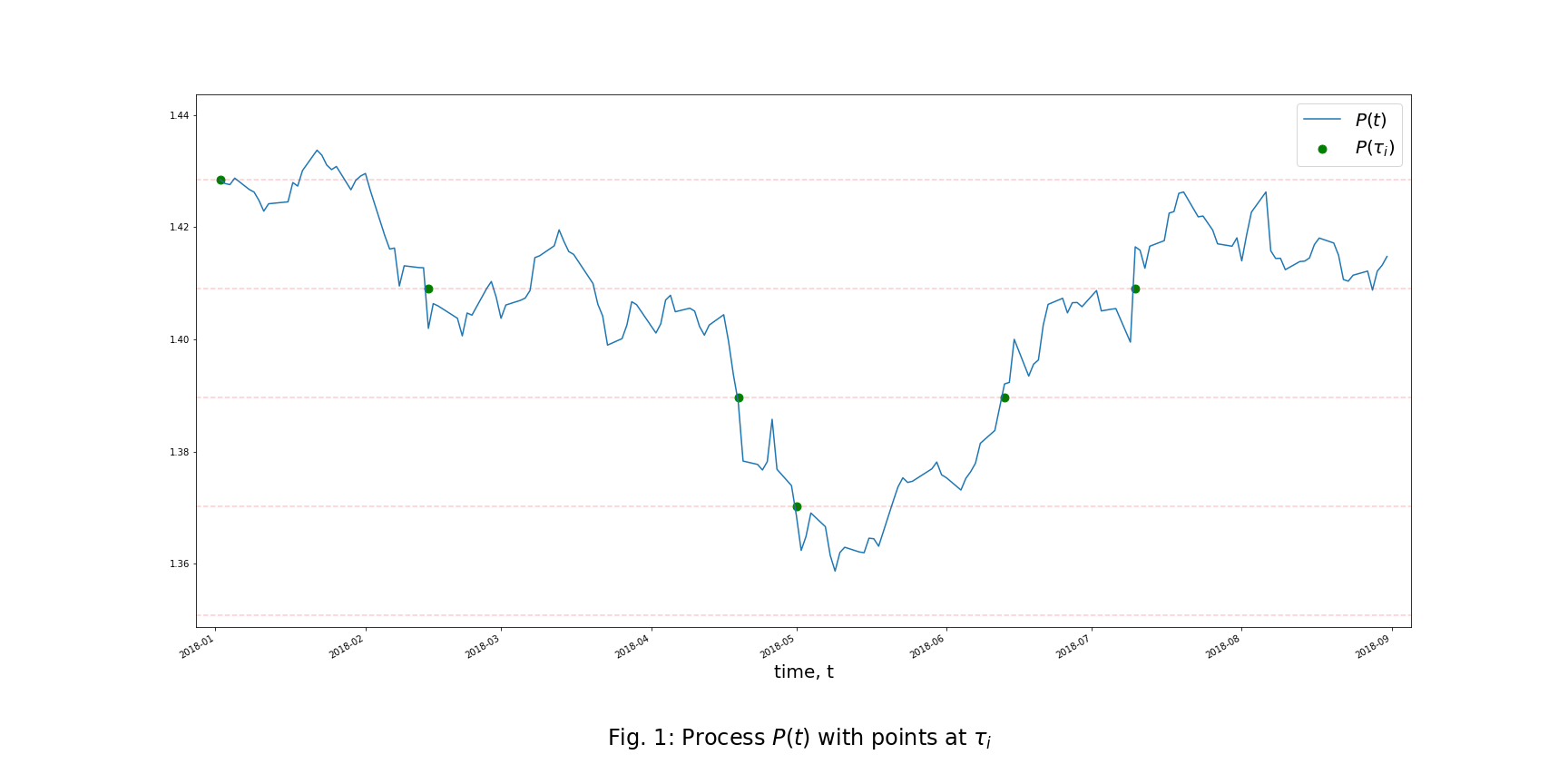
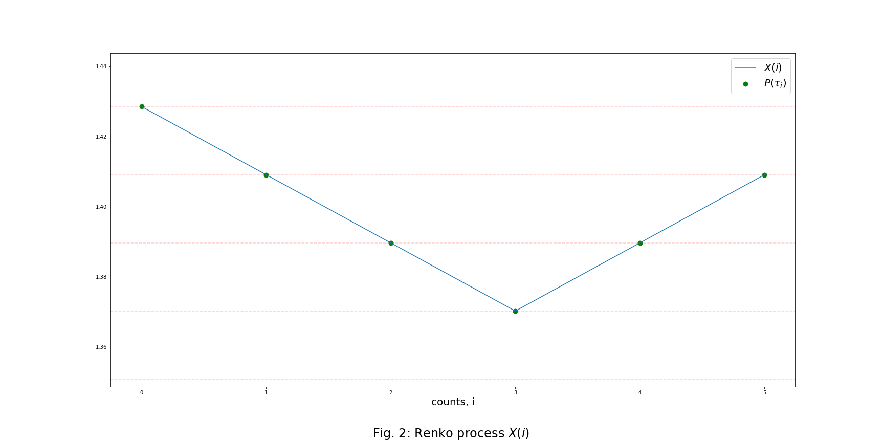
To implement this pairs trading approach, the first thing we must do is to determine the turning points of a tradable process. The paper refers to this decision process as H-construction. There are two types of H-construction, the first is called Renko construction, and the second is called Kagi construction. They correspond to well-known technical analysis tools, Renko chart, and Kagi chart. It is worth noting that the construction processes proposed by the paper are very similar to the ones traditional technical analysis used, but they are slightly different in analytical expressions.

Fig. Renko and Kagi charts.

To start, suppose $P(t)$ is a continuous time series on the time interval $[0, T]$ .

Renko Construction

Step 1: Generate the Renko Process

The Renko process $X(i)$ is defined as,

$X(i) : X(i) = P(\tau_i), i = 0, 1, ..., N,$

where $\tau_i$ , $i = 0, 1, ..., N$ is an increasing sequence of time moments such that

for some arbitrary $H > 0$ , $\tau_0 = 0$ and $P(\tau_0) = P(0)$ ,

$H \leq \max \limits_{t \in [0,T]} P(t) - \min \limits_{t \in [0,T]} P(t),$

$\tau_i = inf\{u \in [\tau_{i - 1}, T] : |P(u) − P(\tau_{i - 1})| = H\}.$

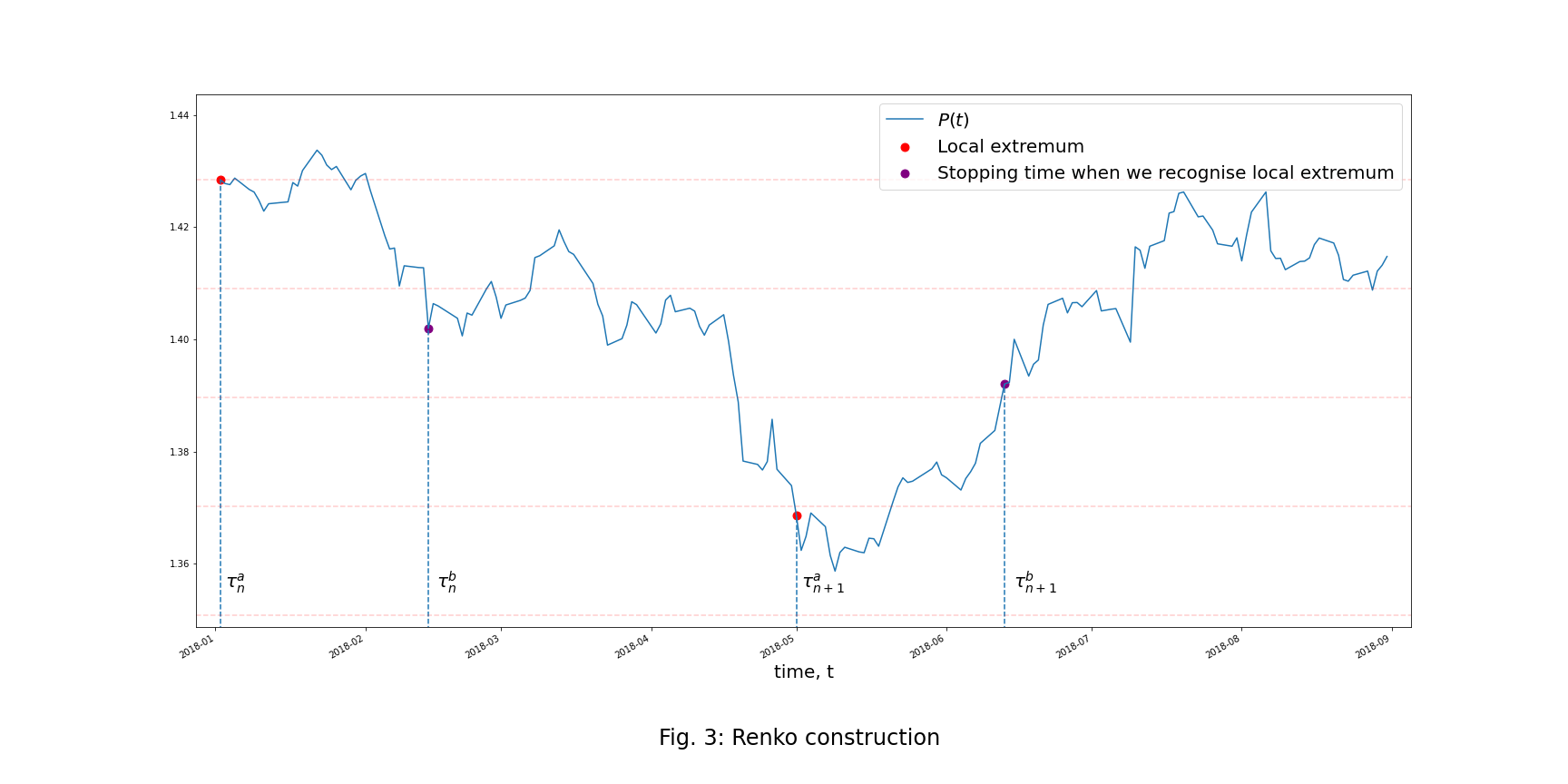
Step 2: Determine Turning Points

We create another sequence of time moments $\{(\tau^a_n, \tau^b_n), n = 0, 1, ..., M\}$ based on the sequence ${\tau_i}$ . The sequence $\{\tau^a_n\}$ defines time moments when the Renko process $X(i)$ has a local maximum or minimum, which means the process $X(i) = P(\tau_i)$ changes its direction and forms a turning point, and the sequence $\{\tau^b_n\}$ defines the time moments when the local maximum or minimum is detected.

More precisely, when we take $\tau^a_0 = \tau_0$ and $\tau^b_0 = \tau_1$ then

$\tau^b_n = min\{\tau_i > \tau^b_{n-1}: (P(\tau_i) - P(\tau_{i-1}))(P(\tau_{i-1}) - P(\tau_{i-2})) < 0\},$

$\tau^a_n = \{\tau_{i - 1} : \tau^b_n = \tau_i\}.$

Kagi Construction

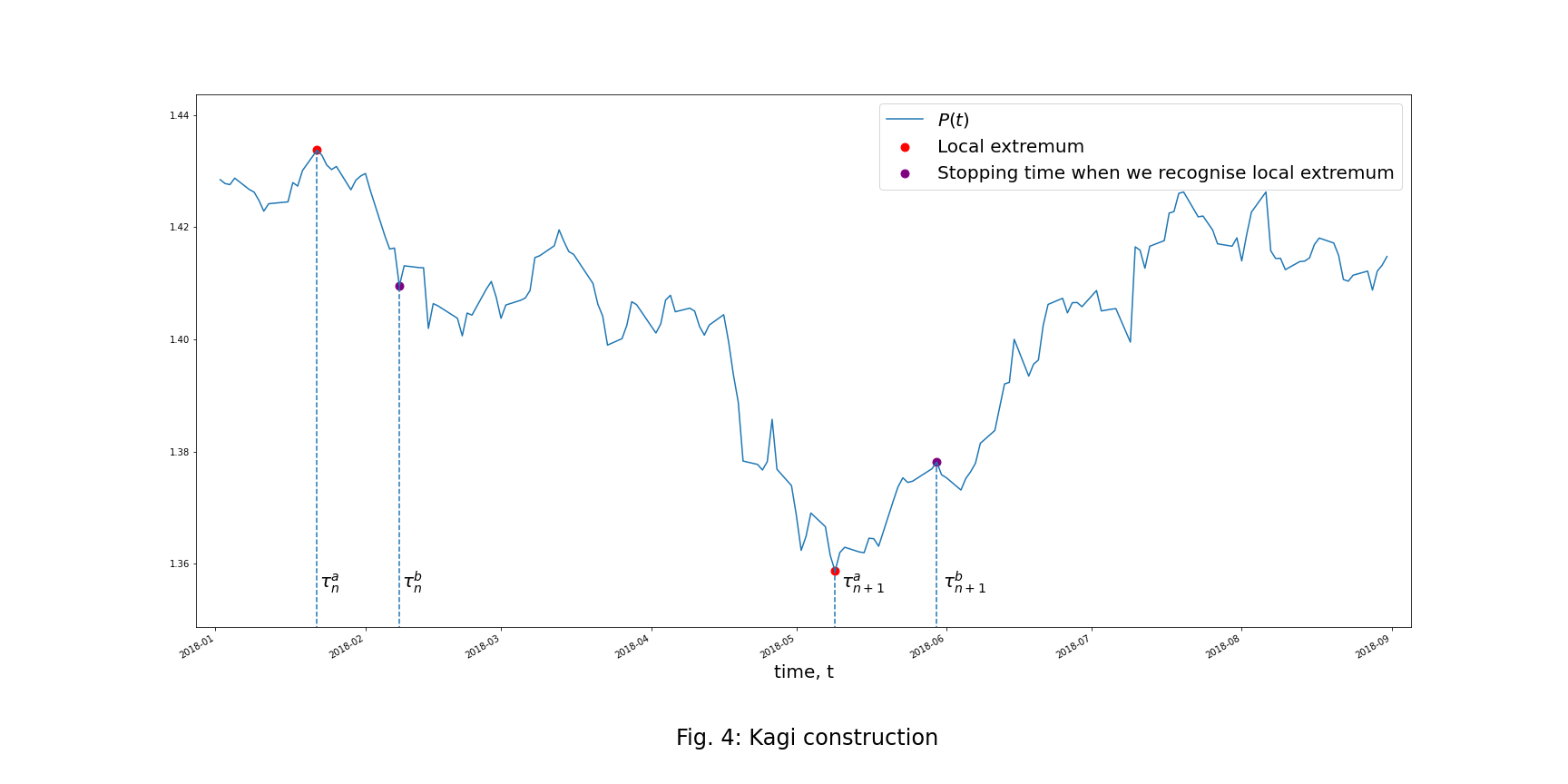
The Kagi construction is similar to the Renko construction with the only difference being that to create the sequence of time moments $\{(\tau^a_n, \tau^b_n), n = 0, 1, ..., M\}$ for the Kagi construction we use local maximums and minimums of the process $P(t)$ rather than the process $X(i)$ derived from it.

The sequence $\{\tau^a_n\}$ then defines the time moments when the price process $P(t)$ has a local maximum or minimum, and the sequence $\{\tau^b_n\}$ defines the time moments when that local maximum or minimum is recognized, which is the time when the process $P(t)$ moves away from its last local maximum or minimum by a distance equal to $H$ .

More precisely, $\tau^a_0$ , $\tau^b_0$ and $S_0$ is defined as,

$\tau^b_0 = inf\{u \in [0, T] : \max \limits_{t \in [0,u]} P(t) − \min \limits_{t \in [0,u]} P(t) = H\},$

$\tau^a_0 = inf\{u < \tau^b_0: |P(u) − P(\tau^b_0)| = H\},$

$S_0 = sign(P(\tau^a_0) − P(\tau^b_0)).$

where $S_0$ can take two values: $1$ for a local maximum and $-1$ for a local minimum.

Then we define $(\tau^a_n, \tau^b_n)$ , $n > 0$ recursively. The construction of the full sequence $\{(\tau^a_n, \tau^b_n), n = 0, 1, ..., M\}$ is done inductively by alternating the following cases.

$Case\ 1: \ \ S_{n-1} = -1$

if $S_{n-1} = -1$ , then $\tau^a_n, \tau^b_n$ and $S_n$ is defined as,

$\tau^b_n = inf\{u \in [\tau^a_{n-1}, T] : P(u) − \min \limits_{t \in [\tau^a_{n-1}\ \ ,\ u]} P(t) = H\},$

$\tau^a_n = inf\{u < \tau^b_n: P(u) = \min \limits_{t \in [\tau^a_{n-1}\ \ ,\ \tau^b_n]} P(t)\},$

$S_n = 1.$

$Case\ 2: \ \ S_{n-1} = 1$

if $S_{n-1} = 1$ , then $\tau^a_n, \tau^b_n$ and $S_n$ is defined as,

$\tau^b_n = inf\{u \in [\tau^a_{n-1}, T] : \max \limits_{t \in [\tau^a_{n-1}\ \ ,\ u]} P(t) - P(u) = H\},$

$\tau^a_n = inf\{u < \tau^b_n: P(u) = \max \limits_{t \in [\tau^a_{n-1}\ \ ,\ \tau^b_n]} P(t)\},$

$S_n = -1.$

H-Statistics

After we’ve determined the turning points of the tradable process, we can calculate some statistics to describe the characteristics of the process.

H-inversion

H-inversion counts the number of times the process $P(t)$ changes its direction for selected $H$ and $T$ . It is straightforward that mean-reverting processes tend to have higher H-inversions, so when we are choosing which pair of assets to trade, the level of H-inversion of their spread is a good metric to use. The higher the H-inversion, the more pair is suitable for a mean-reverting strategy.

Formally, it is calculated as

$N_T (H, P) = \max \{n : \tau^{b}_{n} = T\} = N$

where $H$ denotes the threshold of the H-construction, and $P$ denotes the process $P(t)$ .

H-distance

H-distance counts the sum of vertical distances between local maximums and minimums to the power $p$ .

It is calculated as

$V^p_T (H, P) = \sum_{n = 1}^{N}|P(\tau^a_n) − P(\tau^a_{n−1})|^p$

H-volatility

H-volatility of order p measures the variability of the process $P(t)$ for selected $H$ and $T$ . We can see from the formula that the H-volatility calculates the average distance between adjacent turning points. If the H-volatility is high, the process tends to move in the same direction for a significant amount before turning its direction. Therefore, it’s better to pick a pair with lower H-volatility to be used in a pairs trading strategy.

It is calculated as

$\xi^p_T = {V^p_T (H, P)}/{N_T (H, P)}$

Strategies

Since we’ve can determine the turning points of the selected process and calculate their statistics, we can now explore which trading strategies can be used and how to chose the best suiting strategy based on H-statistics.

Momentum Strategy

The investor buys (sells) an asset at a stopping time $\tau^b_n$ when he or she recognizes that the process passed its previous local minimum (maximum) and the investor expects a continuation of the movement. The signal $s_t$ is given by

$s_t = \left\{\begin{array}{l} +1,\ if\ t = \tau^b_n\ and\ P(\tau^b_n) - P(\tau^a_n) > 0 \\ -1,\ if\ t = \tau^b_n\ and\ P(\tau^b_n) - P(\tau^a_n) < 0 \\ 0,\ otherwise \end{array}\right.$

where $+1$ indicates opening a long trade or closing a short trade, $−1$ indicates opening a short trade or closing a long trade and $0$ indicates holding the previous position.

The profit from one trade according to the momentum H-strategy over time from $\tau^b_{n−1}$ to $\tau^b_{n}$ is

$Y_{\tau^b_n} = (P(\tau^b_n) − P(\tau^b_{n−1})) · sign(P(\tau^a_n) − P(\tau^a_{n−1}))$

and the total profit from time $0$ till time $T$ is

$Y_T(H, P) = (\xi^1_T (H, P) − 2H) \cdot N_T (H, P)$

Contrarian Strategy

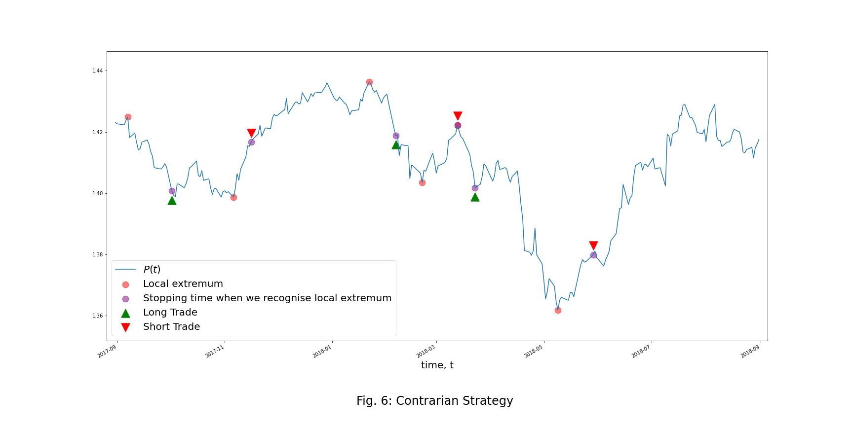
The investor sells (buys) an asset at a stopping time $\tau^b_n$ when he or she decides that the process has passed far enough from its previous local minimum (maximum), and the investor expects a movement reversion. The signal $s_t$ is given by

$s_t = \left\{\begin{array}{l} +1,\ if\ t = \tau^b_n\ and\ P(\tau^b_n) - P(\tau^a_n) < 0 \\ -1,\ if\ t = \tau^b_n\ and\ P(\tau^b_n) - P(\tau^a_n) > 0 \\ 0,\ otherwise \end{array}\right.$

where $+1$ indicates opening a long trade or closing a short trade, $−1$ indicates opening a short trade or closing a long trade and $0$ indicates holding the previous position.

The profit from one trade according to the momentum H-strategy over time from $\tau^b_{n−1}$ to $\tau^b_{n}$ is

$Y_{\tau^b_n} = (P(\tau^b_n) − P(\tau^b_{n−1})) · sign(P(\tau^a_{n−1}) - P(\tau^a_n))$

and the total profit from time $0$ till time $T$ is

$Y_T(H, P) = (2H - \xi^1_T (H, P)) \cdot N_T (H, P)$

Properties

It is clear that the choice of H-strategy depends on the value of H-volatility. If $\xi^1_T > 2H$ , then to achieve a positive profit the investor should employ a momentum H -strategy; if $\xi^1_T < 2H$ then the investor should use a contrarian H-strategy.

Suppose $P(t)$ follows the Wiener process, the H-volatility $\xi^1_T = 2H$ . As a result, it is impossible to profit from the trading on the process. We can also see that H-volatility $\xi^1_T = 2H$ is a property of a martingale. Likewise $\xi^1_T > 2H$ could be a property of a sub-martingale or a super-martingale or a process regularly switching over time from a sub-martingale to a super-martingale and back.

In the reference paper, the author proposes that for any mean-reverting process, regardless of its distribution, the H-volatility is less than $2H$ . Hence, theoretically, trading the mean-reverting process by the contrarian H-strategy is profitable for any choice of $H$ .

Pairs Selection

From the above discussions, we know that using the contrarian strategy applied to a process with mean reversion properties has a high chance of generating a profit. This paper then proposes a straightforward but valuable pairs selection method to find the spread processes with desired mean reversion properties by using the properties of H-inversion.

Purpose: Select trading pairs from the assets pool by using the properties of the H-inversion.
Algorithm:

Determine the assets pool and the length of observed historical data.
Take log-prices of all assets based on the historical data, combine them in all possible pairs and build spread process for each pair.
$spread_{ij} = log(P_i) - log(P_j)$
For each spread process, calculate its historical standard deviation, and set it as the threshold of the H-construction.
Determine the construction type of the H-construction. It could be either Renko or Kagi.
Build the H-construction on the spread series formed by each of the possible pairs.
The top N pairs with the highest H-inversion are used for pairs trading.

Pairs Trading on the S&P 500 index

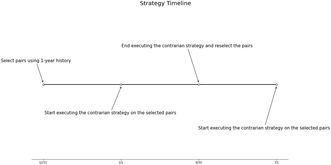
Using the strategy on S&P 500 is proposed by the reference paper, our goal here was to replicate the results of the original work. Every six months, we set the S&P 500 components as our asset pool and use the H-selection method mentioned above to select 20 pairs to be traded. After the selection procedure, we execute the contrarian strategy with these pairs for the next six months. The same thresholds used for the H-selection are also used during the execution of the contrarian trading strategy.

Pairs Selection

Frequency: Reselect every six months.
H-selection parameters:

- Assets pool: S&P 500 Components, updated at the beginning of each year.
- The length of historical data: 12-month history.
- Construction type: Kagi.
- Selection:

- - The top 20 pairs with the highest H-inversion.
  - Not allowing the same asset to appear repeatedly in different pairs.

Trading Strategy

Construction type: Kagi.
Signals type: contrarian.
Trading period: Start trading all pairs from the first day of the trading period and constantly stay in the market for up to six months.

Others

Backtesting interval: 2005/01/01 ~ 2020/07/01
Transaction costs: 2N per trade for the pair and about 4N per round trip for the pair.

Performance

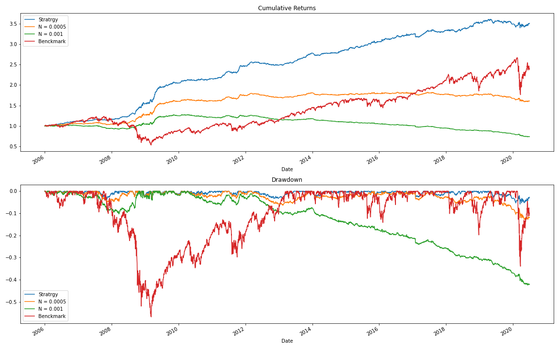
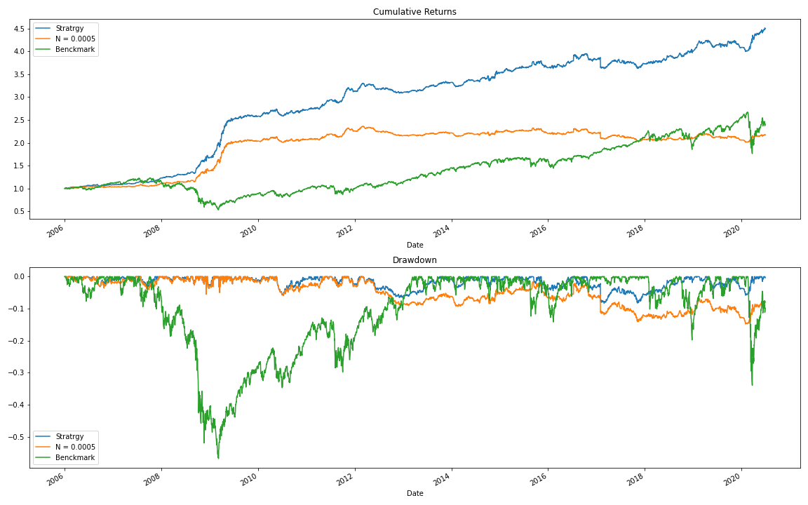
From the results table and the figure below, we can see that performance of the strategy gradually declines over time. However, the results are still good when we have low or moderate transaction costs. One of the reasons for the decline in strategy performance is that the market may gradually become more efficient, making it more challenging to find alpha from a proposed strategy.

What is worth noting is that with moderate transaction costs the strategy is showing significantly lower levels of volatility and Maximum Draw Down, and a Sharpe ratio higher than the benchmark. In this case, we consider the performance of an S&P 500 ETF as a benchmark. Such behavior may pose an interest for more risk-averse traders.

Modification

We mentioned in the above explanation that in theory, when $\xi^1_T < 2H$ , the contrarian strategy can be profitable. We can go further and add a filter to the origin strategy based on the value of the threshold and the H-volatility in the selection period. So now, not only the H-inversion of the selected pair needs to be in the top 20, but also double the threshold value also need to be greater than the sum of the transaction costs and the H-volatility. The constraint described above can be written as,

$\xi^1_T < 2H + 4N$

where $N$ denotes the transaction costs per trade.

We can see from the results table and the chart below that the strategy performance has slightly increased after we added this simple constraint.

N = 0.0005

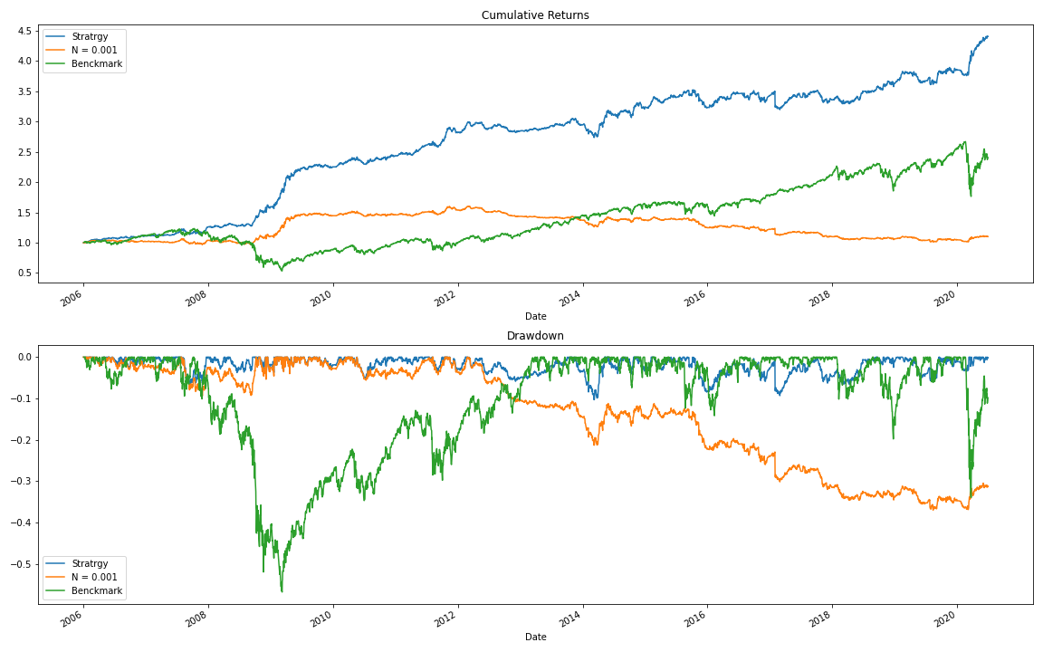
Here are the backtesting results for the modified strategy, but with slightly higher transaction costs. In comparison to the original method, it still stays profitable, even with high transaction costs taken into account.

N = 0.001

Pairs Trading on Cryptocurrencies

Cryptocurrencies have become a trendy trading commodity in recent years. Due to their lack of unique fundamentals to support their value, pairs of cryptocurrencies tend to have a higher and more stable correlation than pairs of stocks. This means they might have qualities needed to be successfully used in pairs trading strategies. Here we simply apply a strategy very similar to the one described in the above section to cryptocurrencies.

Pairs Selection

Frequency: Reselect every 14 days.
H-selection parameters:

- Assets pool: 50 kinds of cryptocurrencies that can be traded on Binance.
- The length of historical data: 28-day history.
- Data Resolution: 4 hours.
- Construction type: Kagi.
- Selection:

- - The top 20 pairs with the highest H-inversion.
  - Twice the threshold value needs to be greater than the sum of the transaction costs and the H-volatility.
  - Allow the same asset to appear repeatedly in different pairs.

Trading Strategy

Construction type: Kagi
Signals type: contrarian.
Trading period: Start trading all pairs from the first day of the trading period and constantly stay in the market for up to 14 days.

Others

Backtesting interval: 2020/01/01 ~ 2021/07/01
Transaction costs: 2N per trade for the pair and about 4N per round trip for the pair.

Performance

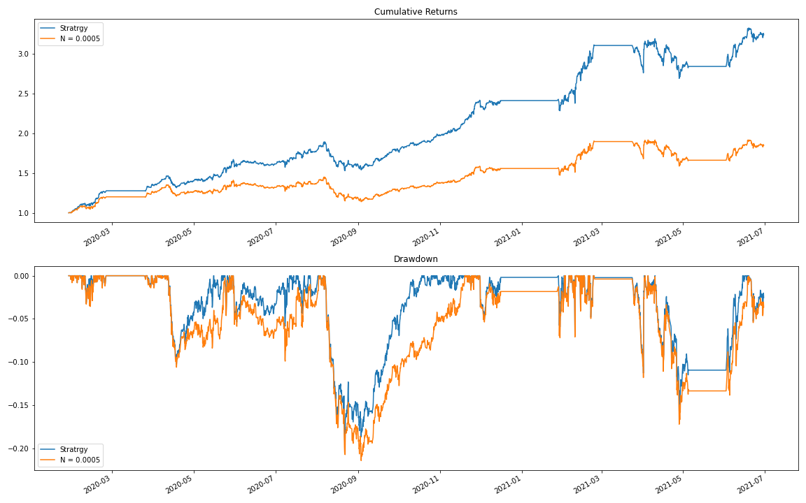
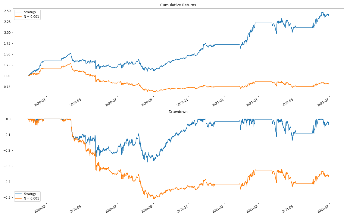
The figure below shows that the performance is acceptable when the transaction costs are 1% per trade for the pair (2N), but is declining when we’re facing a higher level of transaction costs. Unfortunately, the performance does not appear to be stable, based on the cumulative returns plot. One of the reasons for this may be that in recent years, the behavior of the participants in the cryptocurrency market and the supervision rules in various countries have constantly been changing, making the market structure rickety. Also, it should be noted that the question of liquidity was not taken into account when performing this backtest. One might face unexpected price slippages when applying the above strategy to the cryptocurrency market.

N = 0.0005

Here are the trading results when using a higher level of transaction costs. At this level of transaction costs, the strategy is not profitable during the backtest period.

N = 0.001

Conclusion

The paper presented in this article proposed a novel approach to pairs trading based on the idea of Renko and Kagi charts, which is very different from the traditional set of tools used in pairs trading strategies. It was also shown that, theoretically, the contrarian strategy is profitable when applied to a mean-reverting continuous process. Another thing worth mentioning is that the reference paper provides H-statistics that capture the degree of mean reversion and the variability of the process. These properties are essential characteristics for determining which strategy to use and which asset pair to select for trading. Although the strategy performance on S&P 500 components has slightly decayed in recent years, the approach still generates a profit, even with moderate transaction costs, and is showing a good risk profile. Interested readers can apply this strategy to small-cap, medium-cap stocks, or less efficient markets and obtain a more significant result.

Although the overall strategy looks complete, there are still some details that can be improved or further studied:

The way to determine the threshold for the H-construction.

- The approach we mentioned above uses the standard deviation of the historical data as the threshold of the H-construction. However, a more rigorous approach to determine the threshold can be applied. The reference paper suggests that the use of a GARCH model may be promising.

The method for constructing the spread series.

- The paper used $ln(P^A_t) - ln(P^B_t)$ to construct the spread series. One can try other spread series construction methods, like $(P^A_t/P^A_0) - \beta \cdot (P^B_t/P^B_0)$ and $ln(P^A_t/P^A_0) - \beta \cdot ln(P^B_t/P^B_0)$ .

References

- Bogomolov, T., 2013. Pairs trading based on statistical variability of the spread process. Quantitative Finance, 13(9): 1411–1430
- Bogomolov, T., 2010. Pairs Trading in the Land Down Under. SSRN eLibrary.
- Do, B., Faff, R. and Hamza, K., 2006. A New Approach to Modeling and Estimation for Pairs Trading. Monash University, Working Paper.