Portfolio Optimisation with PortfolioLab: Mean-Variance Optimisation
By Aman Dhaliwal and Aditya Vyas
Join the Reading Group and Community: Stay up to date with the latest developments in Financial Machine Learning!
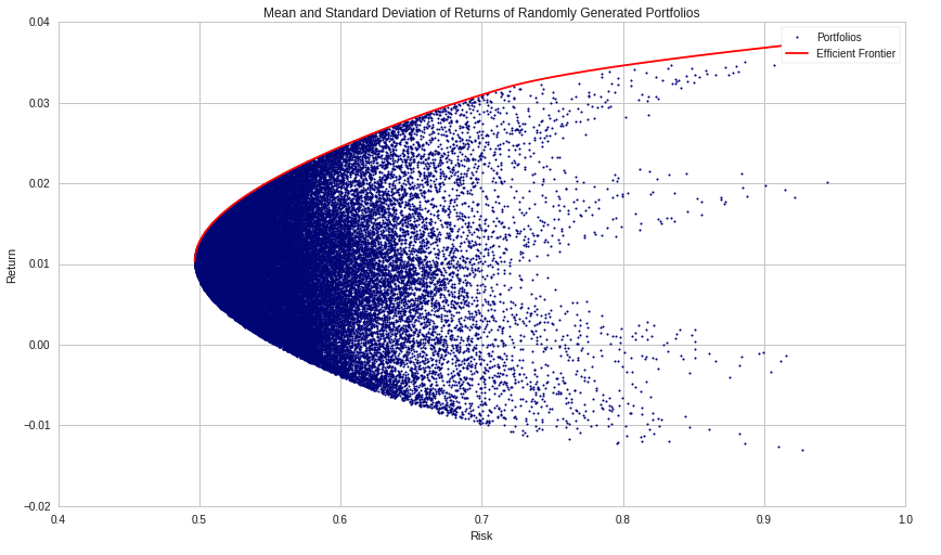
Image Credits: Abasi, Margenot and Granizo-Mackenzie, 2020
For a long while, investors worked under the assumption that the risk and return relationship of a portfolio was linear, meaning that if an investor wanted higher returns, they would have to take on a higher level of risk. This assumption changed when in 1952, Harry Markowitz introduced Modern Portfolio Theory (MPT). MPT introduced the notion that the diversification of a portfolio can inherently decrease the risk of a portfolio. Simply put, this meant that investors could increase their returns while also reducing their risk. Markowitz’s work on MPT was groundbreaking in the world of asset allocation, eventually earning him a Nobel prize for his work in 1990.
Throughout this blog post, we will explore Markowitz’s Modern Portfolio Theory and work through a full implementation in the PortfolioLab library.
Understanding Modern Portfolio Theory
To understand the intuition behind MPT, we must understand that it is a theory at heart. Meaning that it relies on various assumptions which may not always be realistic. It provides a general framework for establishing a range of reasonable expectations of which investors can use to inform their decisions.
Modern Portfolio Theory is based on the following assumptions:
- Investors wish to maximize their utility with a certain level of capital
- Investors have access to fair and correct information of risk and returns
- The markets are efficient
- Investors always try to minimize risk and maximize returns
- Investors prefer the highest returns for a specific level of risk
- Investors base their decisions upon expected returns and the risk of assets
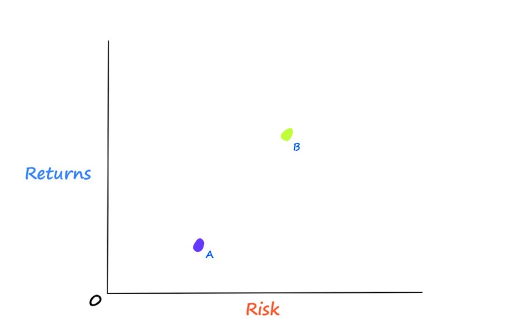
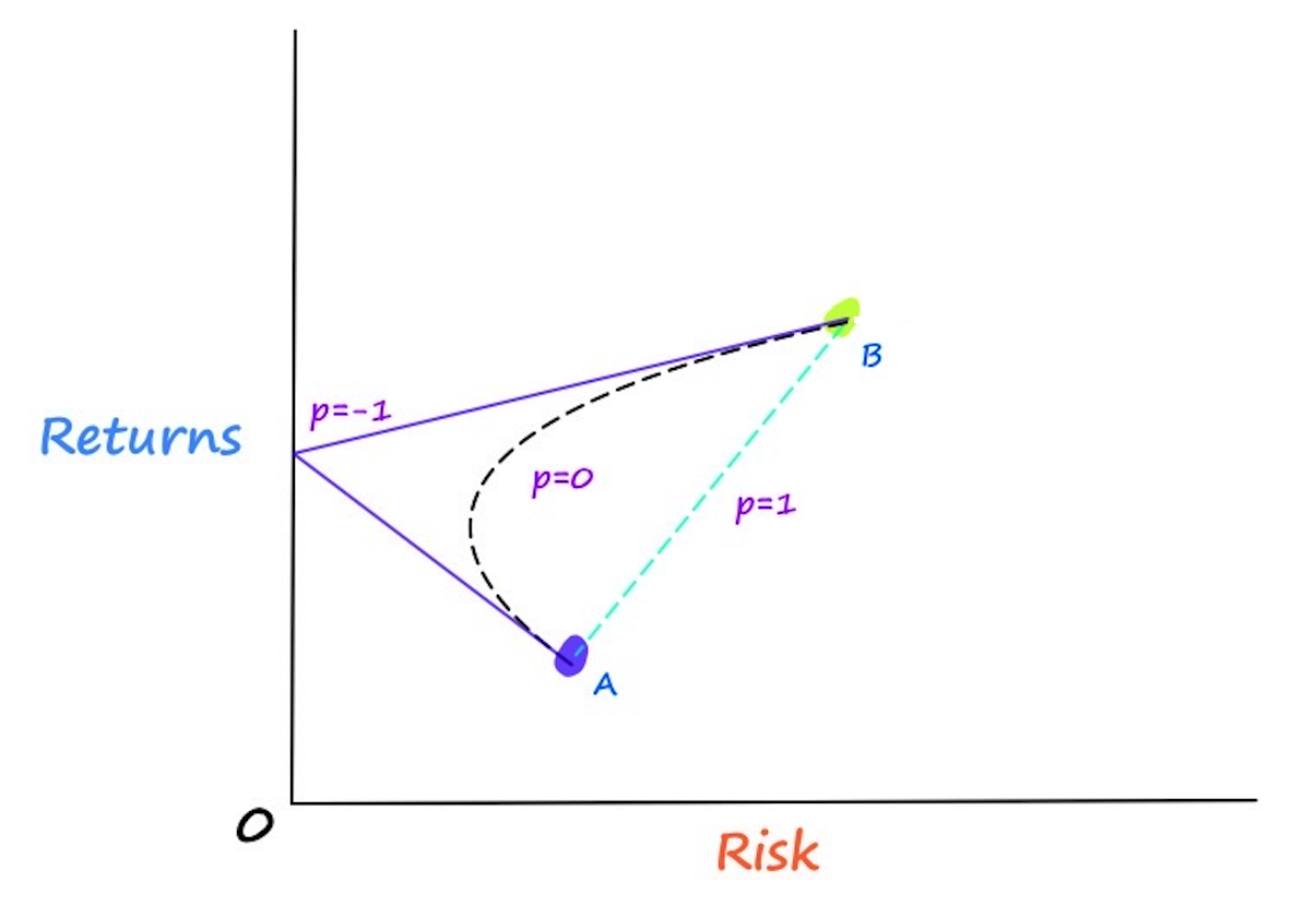
Now that we are familiar with our working assumptions, we can begin to understand the intuition behind MPT. Let’s start by imagining we have two stocks in a portfolio, Stock A and Stock B.
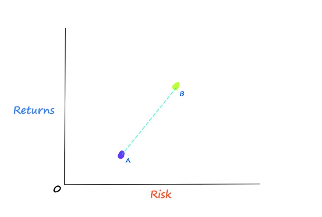
From the image above, we can see how Stock A has a lower expected returns level and a lower risk level than Stock B. Prior to MPT, the possible portfolio combinations between these two stocks was assumed to be linear.
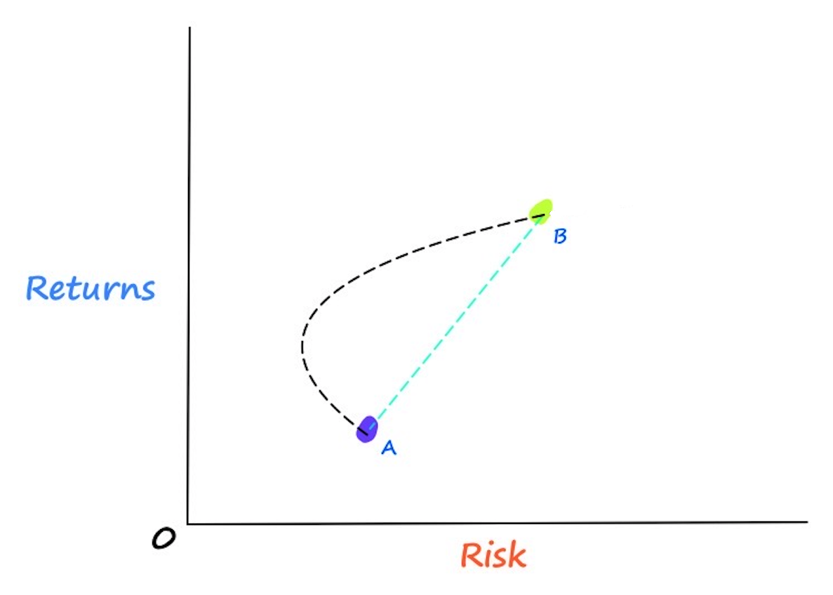
Assuming that there is a linear relationship between our stocks, we would think that all of our possible portfolio combinations would fall somewhere on the dotted line shown above. According to Markowitz, we would be wrong. Markowitz’s theory implies that there is not a linear relationship between our stocks, and that it actually takes a curved shape called the efficient frontier. In which the efficient frontier is the true representation of all our possible portfolio combinations.
So you may now be asking, how is this possible? This efficient frontier is all made possible through a beautiful concept called correlation. To understand how correlation gives us this curved shape representing our portfolio combinations, we first need to understand how our portfolio returns and portfolio risk are calculated.
Portfolio Returns and Risk
In short, the expected return of our portfolio is the proportional sum of our individual assets’ expected returns.\begin{aligned}E(r_p) = \sum_{i=1}^N w_i*E(r_i)\end{aligned} where ![]() is the weight of the
is the weight of the ![]() asset of our portfolio and
asset of our portfolio and ![]() represents the expected return of the
represents the expected return of the ![]() asset of our portfolio.
asset of our portfolio.
This calculation of our portfolio’s expected return follows the same intuition which would make us believe that the relationship between our two stocks would be linear. The part which makes this relationship non-linear comes when calculating our portfolio’s risk.
Now that we can calculate our portfolio’s expected returns, we can see how to calculate our portfolio’s risk, which is represented as our portfolio’s variance.\begin{aligned}\sigma_p^2 = w_A^2\sigma_A^2 + w_B^2\sigma_B^2 + 2 w_A w_B \sigma_A \sigma_B \rho_{A,B}\end{aligned} where ![]() represents our correlation between stocks and
represents our correlation between stocks and represents the standard deviation for each stock. Now that we can see how our risk equation is affected by the correlation between our two stocks, we can begin to understand why we get an efficient frontier shape for our possible portfolio combinations.
The correlation of our two assets is a number between -1 and 1 which shows us how our two stocks are related. If our correlation is positive, the returns of our two assets tend to move in the same direction, and vice versa. To calculate the correlation of Stock A and Stock B, it would look like this:\begin{aligned}corr_{A,B} = \rho_{A,B} = \frac{\sigma_{A,B}}{\sigma_A\sigma_B}\end{aligned} where ![]() represents our covariance between stocks A and B.
represents our covariance between stocks A and B.
Looking at our calculation for the portfolio risk above, we can see that when the correlation of our stocks is negative, it reduces our overall portfolio risk, while it does not affect our portfolio’s expected return. To understand this a little better, let’s go back to our example.
Looking at the picture above, it showcases three different scenarios. When the correlation between our two stocks is -1, there is the largest reduction in our portfolio risk. Meanwhile, as the correlation between our stocks increases, our portfolio risk increases as well.
While this was intended as a quick primer on Modern Portfolio Theory, we hope this gives you a basic understanding of the topic for which you can further read upon. There are lots of great articles and papers written on the subject that go into the depth of the topic. The rest of this blog post will be geared towards implementing this portfolio optimisation technique through the PortfolioLab library.
Supported Portfolio Allocation Solutions
The MPT or Mean-Variance Optimisation encompasses a large variety of portfolio solutions with different objectives and constraints. The MeanVarianceOptimisation class provides some of these commonly encountered portfolio problems out-of-the-box:
Inverse Variance
For this solution, the diagonal of the covariance matrix is used for weights allocation.\begin{aligned}w_{i} = \frac{\sum^{-1}}{\sum_{j=1}^{N}(\sum_{j,j})^{-1}}\end{aligned}
where ![]() is the weight allocated to the
is the weight allocated to the ![]() asset in a portfolio,
asset in a portfolio, ![]() is the
is the ![]() element on the main diagonal of the covariance matrix of elements in a portfolio and
element on the main diagonal of the covariance matrix of elements in a portfolio and ![]() is the number of elements in a portfolio.
is the number of elements in a portfolio.
Minimum Volatility
For this solution, the objective is to generate a portfolio with the least variance. The following optimization problem is being solved.\begin{aligned}& \underset{\mathbf{w}}{\text{minimise}} & & w^T\sum w \\ & \text{s.t.} & & \sum_{j=1}^{n}w_{j} = 1 \\ &&& w_{j} \geq 0, j=1,..,N \end{aligned}
Maximum Sharpe Ratio
For this solution, the objective is (as the name suggests) to maximise the Sharpe Ratio of your portfolio.\begin{aligned} & \underset{\mathbf{w}}{\text{maximise}} & & \frac{\mu^{T}w – R_{f}}{(w^{T}\sum w)^{1/2}} \\ & \text{s.t.} & & \sum_{j=1}^{n}w_{j} = 1 \\ &&& w_{j} \geq 0, j=1,..,N \end{aligned}
A major problem with the above formulation is that the objective function is not convex and this presents a problem for cvxpy which only accepts convex optimization problems. As a result, the problem can be transformed into an equivalent one, but with a convex quadratic objective function.\begin{aligned} & \underset{\mathbf{w}}{\text{minimise}} & & y^T\sum y \\ & \text{s.t.} & & (\mu^{T}w – R_{f})^{T}y = 1 \\ &&& \sum_{j=1}^{N}y_{j} = \kappa, \\ &&& \kappa \geq 0, \\ &&& w_{j} = \frac{y_j}{\kappa}, j=1,..,N \end{aligned}
where ![]() refer to the set of unscaled weights,
refer to the set of unscaled weights, ![]() is the scaling factor and the other symbols refer to their usual meanings.
is the scaling factor and the other symbols refer to their usual meanings.
The process of deriving this optimization problem from the standard maximising Sharpe ratio problem is described in the notes IEOR 4500 Maximizing the Sharpe ratio from Columbia University.
Efficient Risk
For this solution, the objective is to minimise risk given a target return value by the investor. Note that the risk value for such a portfolio will not be the minimum, which is achieved by the minimum-variance solution. However, the optimiser will find the set of weights which efficiently allocate risk constrained by the provided target return, hence the name “efficient risk”.\begin{aligned} & \underset{\mathbf{w}}{\text{min}} & & w^T\sum w \\ & \text{s.t.} & & \mu^Tw = \mu_t\\ &&& \sum_{j=1}^{n}w_{j} = 1 \\ &&& w_{j} \geq 0, j=1,..,N \\ \end{aligned}
where ![]() is the target portfolio return set by the investor and the other symbols refer to their usual meanings.
is the target portfolio return set by the investor and the other symbols refer to their usual meanings.
Efficient Return
For this solution, the objective is to maximise the portfolio return given a target risk value by the investor. This is very similar to the efficient_risk solution. The optimiser will find the set of weights which efficiently try to maximise return constrained by the provided target risk, hence the name “efficient return”.\begin{aligned} & \underset{\mathbf{w}}{\text{max}} & & \mu^Tw \\ & \text{s.t.} & & w^T\sum w = \sigma^{2}_t\\ &&& \sum_{j=1}^{n}w_{j} = 1 \\ &&& w_{j} \geq 0, j=1,..,N \\ \end{aligned}
where ![]() is the target portfolio risk set by the investor and the other symbols refer to their usual meanings.
is the target portfolio risk set by the investor and the other symbols refer to their usual meanings.
Maximum Return – Minimum Volatility
This is often referred to as quadratic risk utility. The objective function consists of both the portfolio return and the risk. Thus, minimising the objective relates to minimising the risk and correspondingly maximising the return. Here, \lambda is the risk-aversion parameter which models the amount of risk the user is willing to take. A higher value means the investor will have high defense against risk at the expense of lower returns and keeping a lower value will place higher emphasis on maximising returns, neglecting the risk associated with it.\begin{aligned} & \underset{\mathbf{w}}{\text{min}} & & \lambda * w^T\sum w – \mu^Tw\\ & \text{s.t.} & & \sum_{j=1}^{n}w_{j} = 1 \\ &&& w_{j} \geq 0, j=1,..,N \\ \end{aligned}
Maximum Diversification
Maximum diversification portfolio tries to diversify the holdings across as many assets as possible. In the 2008 paper, Toward Maximum Diversification, the diversification ratio, D, of a portfolio, is defined as:\begin{aligned}D = \frac{w^{T}\sigma}{\sqrt{w^{T}\sum w}}\end{aligned}
where ![]() is the vector of volatilities and
is the vector of volatilities and ![]() is the covariance matrix. The term in the denominator is the volatility of the portfolio and the term in the numerator is the weighted average volatility of the assets. More diversification within a portfolio decreases the denominator and leads to a higher diversification ratio. The corresponding objective function and the constraints are:\begin{aligned} & \underset{\mathbf{w}}{\text{max}} & & D\\ & \text{s.t.} & & \sum_{j=1}^{n}w_{j} = 1 \\ &&& w_{j} \geq 0, j=1,..,N \\ \end{aligned}
is the covariance matrix. The term in the denominator is the volatility of the portfolio and the term in the numerator is the weighted average volatility of the assets. More diversification within a portfolio decreases the denominator and leads to a higher diversification ratio. The corresponding objective function and the constraints are:\begin{aligned} & \underset{\mathbf{w}}{\text{max}} & & D\\ & \text{s.t.} & & \sum_{j=1}^{n}w_{j} = 1 \\ &&& w_{j} \geq 0, j=1,..,N \\ \end{aligned}
You can read more about maximum diversification portfolio in the following blog post on the website Flirting with Models: Maximizing Diversification.
Maximum Decorrelation
For this solution, the objective is to minimise the correlation between the assets of a portfolio\begin{aligned} & \underset{\mathbf{w}}{\text{min}} & & w^TA w\\ & \text{s.t.} & & \sum_{j=1}^{n}w_{j} = 1 \\ &&& w_{j} \geq 0, j=1,..,N \\ \end{aligned}
where ![]() is the correlation matrix of assets. The Maximum Decorrelation portfolio is closely related to Minimum Variance and Maximum Diversification, but applies to the case where an investor believes all assets have similar returns and volatility, but heterogeneous correlations. It is a Minimum Variance optimization that is performed on the correlation matrix rather than the covariance matrix,
is the correlation matrix of assets. The Maximum Decorrelation portfolio is closely related to Minimum Variance and Maximum Diversification, but applies to the case where an investor believes all assets have similar returns and volatility, but heterogeneous correlations. It is a Minimum Variance optimization that is performed on the correlation matrix rather than the covariance matrix, ![]() .
.
You can read more on maximum decorrelation portfolio in the following blog post: Max Decorrelation Portfolio.
Mean-Variance Optimisation with PortfolioLab
In this section, we will show users how to optimize their portfolio using several mean-variance optimisation (MVO) solutions provided through the PortfolioLab Python library. Official documentation can be found at this link. The mean-variance optimisation class from PortfolioLab utilizes techniques based on Harry Markowtiz’s methods for calculating efficient frontier solutions. Through the PortfolioLab library, users can generate optimal portfolio solutions for different objective functions, including:
# importing our required libraries
import pandas as pd
import numpy as np
import matplotlib.pyplot as plt
from portfoliolab.modern_portfolio_theory import MeanVarianceOptimisation
The Data
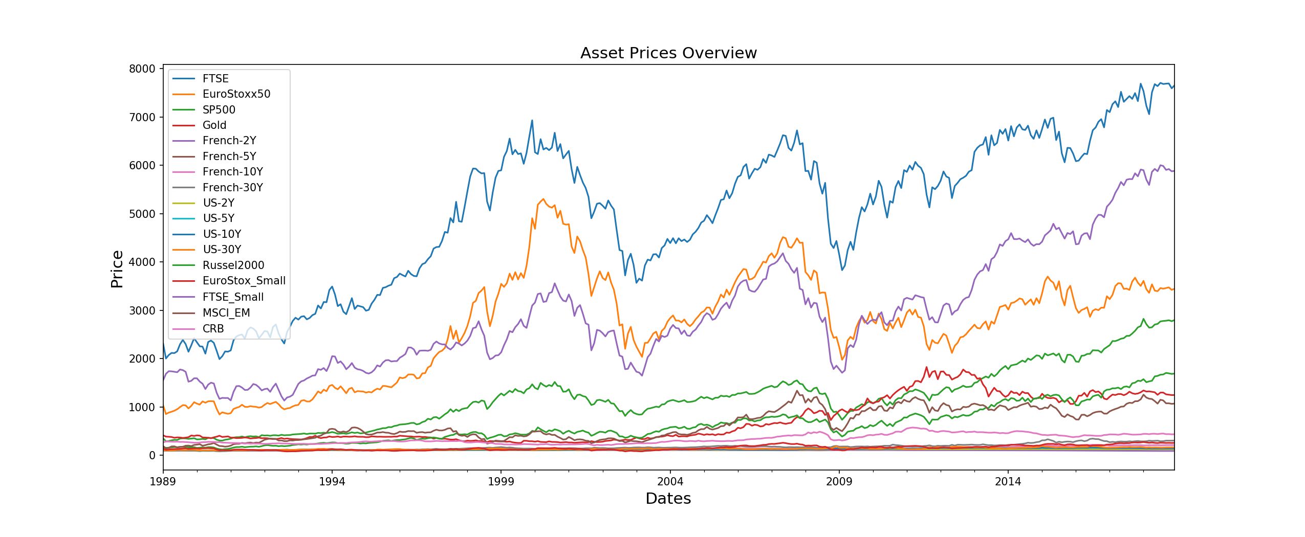
In this tutorial, we will be working with the historical closing prices for 17 assets. The portfolio consists of diverse set of assets ranging from commodities to bonds and each asset exhibits different risk-return characteristics. You can download the dataset CSV file from our research repository here
# preparing our data
raw_prices = pd.read_csv('../Sample-Data/assetalloc.csv', sep=';', parse_dates=True, index_col='Dates')
stock_prices = raw_prices.sort_values(by='Dates')

# Taking a quick look at our most recent 5000 data points
stock_prices.resample('M').last().plot(figsize=(17,7))
plt.ylabel('Price', size=15)
plt.xlabel('Dates', size=15)
plt.title('Stock Data Overview', size=15)
plt.show()
Calculating some Example Portfolios
We will first work through building an optimal portfolio under the inverse-variance solution string. It is one of the simplest yet powerful allocation strategy which outperforms a lot of complex optimisation objectives.
In order to calculate the asset weights of the inverse-variance portfolio, we will need to create a new MeanVarianceOptimisation object and use the allocate method. More information on inverse-variance solutions can be found here.
Note that the allocate method requires three parameters to run:
- asset_names (a list of strings containing the asset names)
- asset_prices (a dataframe of historical asset prices – daily close)
- solution (the type of solution/algorithm to use to calculate the weights)
Instead of providing historical asset prices, users can also provide the expected asset returns along with a covariance matrix of asset returns. There is also much more customizability within the allocation method in which we will explore later in this post. For simplicity, we will show users how to create an optimal portfolio under the Inverse Variance portfolio solution. If you wish to create a different optimized portfolio, all that must be changed is the ‘solution’ parameter string. The corresponding solution strings and portfolio solutions can be found at the official documentation.
# creating our portfolio weights under the correct objective function
mvoIV = MeanVarianceOptimisation()
mvoIV.allocate(asset_names=stock_prices.columns,
               asset_prices=stock_prices,
               solution='inverse_variance')

# plotting our optimal portfolio
IV_weights = mvoIV.weights
y_pos = np.arange(len(IV_weights.columns))

plt.figure(figsize=(25,7))
plt.bar(list(IV_weights.columns), IV_weights.values[0])
plt.xticks(y_pos, rotation=45, size=10)
plt.xlabel('Assets', size=20)
plt.ylabel('Asset Weights', size=20)
plt.title('Inverse-Variance Portfolio', size=20)
plt.show()
Let us create another portfolio – the maximum Sharpe Ratio portfolio. This is sometimes also referred to as the tangency portfolio.
# creating our portfolio weights under the correct objective function
mvoMS = MeanVarianceOptimisation()
mvoMS.allocate(asset_names=stock_prices.columns,
                asset_prices=stock_prices,
                solution='max_sharpe')

# plotting our optimal portfolio
MS_weights = mvoMS.weights
y_pos = np.arange(len(MS_weights.columns))

plt.figure(figsize=(25,7))
plt.bar(list(MS_weights.columns), MS_weights.values[0])
plt.xticks(y_pos, rotation=45, size=20)
plt.xlabel('Assets', size=20)
plt.ylabel('Asset Weights', size=20)
plt.title('Maximum Sharpe Portfolio', size=20)
plt.show()
Custom Input from Users
While PortfolioLab provides many of the required calculations when constucting optimal portfolios, users also have the choice to provide custom input for their calculations. Instead of providing the raw historical closing prices for their assets, users can input a covariance matrix of asset returns and the expected asset returns to calculate their optimal portfolio. If you would like to learn more about the customizbility within PortfolioLab’s MVO implementation, please refer to the official documentation.
The following parameters in the allocate() method are utilized in order to do so:
- ‘covariance_matrix’: (pd.DataFrame/NumPy matrix) A covariance matrix of asset returns
- ‘expected_asset_returns: (list) A list of mean asset returns
To make some of the necessary calculations, we will make use of the ReturnsEstimators class provided by PortfolioLab.
# Importing ReturnsEstimation class from PortfolioLab
from portfoliolab.estimators import ReturnsEstimators

# Calculating our asset returns in order to calculate our covariance matrix
returns = ReturnsEstimators.calculate_returns(stock_prices)

# Calculating our covariance matrix
cov = returns.cov()
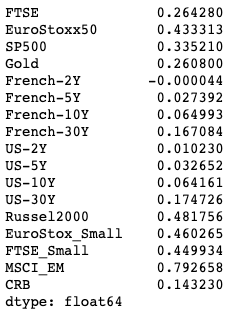
We also calculate the expected returns i.e. mean asset returns
# Calculating our mean asset returns
mean_returns = ReturnsEstimators.calculate_mean_historical_returns(stock_prices)
mean_returns
Having calculated all the required input matrices, we create an efficient risk portfolio using these custom inputs. An efficient risk portfolio tries to efficiently manage risk for a given target return by the investor. Here we are specifying a target return of 0.2
# From here, we can now create our portfolio
mvo_custom = MeanVarianceOptimisation()
mvo_custom.allocate(asset_names=stock_prices.columns,
                    expected_asset_returns=mean_returns,
                    covariance_matrix=cov,
                    target_returns=0.2,
                    solution='efficient_risk')

# plotting our optimal portfolio
custom_weights = mvo_custom.weights
y_pos = np.arange(len(custom_weights.columns))

plt.figure(figsize=(25,7))
plt.bar(list(custom_weights.columns), custom_weights.values[0])
plt.xticks(y_pos, rotation=45, size=20)
plt.xlabel('Assets', size=20)
plt.ylabel('Asset Weights', size=20)
plt.title('Custom MVO Portfolio - Efficient Risk Solution', size=20)
plt.show()
Additionally, a lot of investors and portfolio managers like to place specific weight bounds on some assets in their portfolio. For instance, in the above portfolio, one may want to limit the weights assigned to French-2Y and US-30Y. Let us try to decrease their allocations and diversify the portfolio a little. We place a maximum bound on their weights and a minimum bound on French-5Y and French-10Y. Note that the indexing starts from 0.
mvo_custom_bounds = MeanVarianceOptimisation()
mvo_custom_bounds.allocate(asset_prices=stock_prices,
                           weight_bounds=["weights[4] <= 0.2", "weights[11] <= 0.1", "weights[5] >= 0.05", "weights[6] >= 0.05"],
                           solution='efficient_risk')

# plotting our optimal portfolio
custom_bounds_weights = mvo_custom_bounds.weights
y_pos = np.arange(len(custom_bounds_weights.columns))

plt.figure(figsize=(25,7))
plt.bar(list(custom_bounds_weights.columns), custom_bounds_weights.values[0])
plt.xticks(y_pos, rotation=45, size=20)
plt.xlabel('Assets', size=20)
plt.ylabel('Asset Weights', size=20)
plt.title('Custom MVO Portfolio - Efficient Risk Solution with Weight Bounds', size=20)
plt.tight_layout()
plt.savefig("mvo_custom_weight_bounds.png", dpi=150)
plt.show()
You can see how the weight bounds help us achieve a more diversified portfolio and prevent the weights from becoming too concentrated on only some assets.
Custom Portfolio Allocation with a Custom Objective Function
PortfolioLab also provides a way for users to create their custom portfolio problem. This includes complete flexibility to specify the input, optimization variables, objective function, and the corresponding constraints. In this section, we will work through how to build a custom portfolio allocation with a custom objective function.
The Quadratic Optimizer
In order to solve our mean-variance objective functions, PortfolioLab uses cvxpy instead of the more frequently used scipy.optimize. This choice was made for a few reasons in particular:
- The documentation of cvxpy is more understandable than that of scipy
- cvxpy’s code is much more readable and easier to understand
- cvxpy raises clear error notifications if the problem we are attempting to solve is not convex and the required conditions are not met
Working with cvxpy through the PortfolioLab library, we can create our own convex optimization function to solve for portfolio allocation. In order to build this custom portfolio, we must follow the general steps:
- Specifying our input variables not related to cvxpy
- Specifying our cvxpy specific variables
- Specifying our objective function
- (Optional) Specifying the constrains for our optimization problem
Step-1: Specifying our variables not related to cvxpy
In this step we must specify our input variables not related to cvxpy (i.e. not defined as cvxpy variable objects). This can include anything ranging from raw asset prices data to historical returns to integer or string variables. All data types are supported in this step – int, float, str, Numpy matrices/lists, Python lists, Pandas DataFrame).
non_cvxpy_variables = {
    'asset_prices': stock_prices,
    'num_assets': stock_prices.shape[1],
    'covariance': stock_prices.cov(),
    'asset_names': stock_prices.columns,
    'expected_returns': mean_returns
}
Step-2: Specifying our cvxpy specific variables
The second step is to specify the cvxpy specific variables which are declared in the syntax required by cvxpy. You can include as many new variables as you need by initialising a simple Python list with each declaration being a string. Each of these variables should be a cvxpy.Variable object.
cvxpy_variables = [
        'risk = cp.quad_form(weights, covariance)',
        'portfolio_return = cp.matmul(weights, expected_returns)'
]
Here, we are declaring two new cvxpy variables – ‘risk’ and ‘portfolio_return’. Note that we are using non-cvxpy variables – ‘covariance’ and ‘expected_returns’ – declared in the previous step to initialise the new ones.
Step-3: Specifying our objective function
The third step is to specify the objective function for our portfolio optimization problem. You need to simply pass a string form of the Python code for the objective function.
custom_obj = 'cp.Minimize(risk)'
Step-4: Specifying the constraints for our optimization problem
This is an optional step which requires you to specify the constraints for your optimization problem. Similar to how we specified cvxpy variables, the constraints need to be specified as a Python list with each constraint being a string representation.
constraints = ['cp.sum(weights) == 1', 'weights >= 0', 'weights <= 1']
Piecing our four parts together, we can now build our custom portfolio allocation.
mvo_custom_portfolio = MeanVarianceOptimisation()
mvo_custom_portfolio.allocate_custom_objective(non_cvxpy_variables=non_cvxpy_variables,
                                               cvxpy_variables=cvxpy_variables,
                                               objective_function=custom_obj,
                                               constraints=constraints)

# plotting our optimal portfolio
mvo_custom_weights = mvo_custom_portfolio.weights
y_pos = np.arange(len(mvo_custom_weights.columns))

plt.figure(figsize=(25,7))
plt.bar(list(mvo_custom_weights.columns), mvo_custom_weights.values[0])
plt.xticks(y_pos, rotation=45, size=10)
plt.xlabel('Assets', size=20)
plt.ylabel('Asset Weights', size=20)
plt.title('Custom Portfolio with Custom Objective Function', size=20)
plt.show()
Conclusion and Further Reading
Throughout this blog post, we explored the intuition behind Harry Markowitz's Modern Portfolio Theory and the relationship behind portfolio risk and return and how it relates to the efficient frontier. PortfolioLab's MeanVarianceOptimisation class provides users with the ability to create some standard portfolios out-of-the-box. At the same time, a lot of flexibility is provided for someone wanting to create their own optimisation problems with custom objective, data and constraints. If you want to read more about the literature and delve deeper into the theory, here are some links to good online resources which might be useful.

