An Introduction to Cointegration for Pairs Trading

By Yefeng Wang

Join the Reading Group and Community: Stay up to date with the latest developments in Financial Machine Learning!

LEARN MORE ABOUT PAIRS TRADING STRATEGIES WITH “THE DEFINITIVE GUIDE TO PAIRS TRADING”

Introduction

Cointegration, a concept that helped Clive W.J. Granger win the Nobel Prize in Economics in 2003 (see Footnote 1), is a cornerstone of pairs and multi-asset trading strategies. Anecdotally, forty years have passed since Granger coined the term “cointegration” in his seminal paper “Some properties of time series data and their use in econometric model specification” (Granger, 1981), yet one still cannot find the term in Merriam-Webster, and some spell checkers will draw a wavy line without hesitation beneath its every occurrence.

Indeed, the concept of cointegration is not immediately apparent from its name. Therefore, in this article, I will attempt to answer the following questions:

What does “integration” in the word “cointegration” refer to?
What are some intuitive interpretations of cointegrated time series?
How to construct a stationary spread from two non-stationary price series?
How to simulate a cointegrated asset pair from scratch?

Hopefully, after reading this article, you will understand better why cointegration techniques, which were initially intended to avoid spurious regression results when using non-stationary regressors in macroeconomic time series analysis (McDermott, 1990), became an indispensable member of the statistical arbitrage arsenal. I will try my best to cut down the amount of hypnotizing math formulae as intuition is more important. Let’s dive in!

What is Cointegration?

Is it $\int f(x) \, dx$ ? I have to admit that every time I read about cointegration, the integral symbol would always pop into my head. But no, cointegration has nothing to do with the integral symbol.

The word “integration” refers to an integrated time series of order d, denoted by $I(d)$ . According to Alexander et al. (Alexander, 2002), price, rate, and yield data can be assumed as $I(1)$ series, while returns (obtained by differencing the price) can be assumed as $I(0)$ series (see Footnote 2). The most important property of the $I(0)$ series that is relevant to statistical arbitrage is the following:

$I(0)$ series are weak-sense stationary

Weak-sense stationarity implies that the mean and the variance of the time series are finite and do not change with time. Mathematically, a stricter definition of stationary, or strict-sense stationary exists, but for financial applications, weak-sense stationarity is sufficient. Therefore, in the remaining part of this article, I will simply use “stationary” to refer to weak-sense stationary series.

This is great news. We found a time-invariant property, which is the mean of the time series. This implies the behavior of the time series has become more predictable, for if the time series wanders too far away from the mean, the time-invariant property will “drag” the series back to make sure the mean does not change. Sounds like we just described a mean-reversion strategy.

But wait, the $I(0)$ series is the returns: we cannot trade the returns! Only the price is tradable, yet the price is an $I(1)$ series, which are not stationary. We cannot make use of the stationary property of the $I(0)$ series by trading one asset.

What about two assets? According to the definition of cointegration (Alexander, 2002):

$x_t$ and $y_t$ are cointegrated, if $x_t$ and $y_t$ are $I(1)$ series and $\exists \, \beta$ such that $z_t = x_t - \beta y_t$ is an $I(0)$ series

Voilà! Cointegration allows us to construct a stationary time series from two asset price series, if only we can find the magic weight, or more formally, the cointegration coefficient $\beta$ . Then we can apply a mean-reversion strategy to trade both assets at the same time weighted by $\beta$ . There is no guarantee that such $\beta$ always exists, and you should look for other asset pairs if no such $\beta$ can be found.

Intuitive Interpretation of Cointegration

Looks like our work is done if we figure out how to find the cointegration coefficient. But before we get gung-ho about $\beta$ , it is helpful to establish an intuitive understanding of the definition of cointegration.

Going back to the definition, we have two $I(1)$ series, $x_t$ and $y_t$ , and they are cointegrated. Now we decompose $x_t$ and $y_t$ into a nonstationary component $\nu$ and a stationary component $\varepsilon$ as follows (Vidyamurthy, 2004):

\begin{alignat*}{2}
x_t &= \nu_{x_t} + \varepsilon_{x_t} \\
y_t &= \nu_{y_t} + \varepsilon_{y_t}
\end{alignat*}

Now we construct the cointegrated series $z_t$ , or the spread between $x_t$ and $y_t$ , with the cointegration coefficient $\beta$ :

\begin{alignat*}{2}
z_t = x_t – \beta y_t = (\nu_{x_t} – \beta \nu_{y_t}) + (\varepsilon_{x_t} – \varepsilon_{y_t})
\end{alignat*}

The definition made clear that $z_t$ is an $I(0)$ process, which indicates $\nu_{x_t} = \beta \nu_{y_t}$ , as there can be no nonstationary component in a stationary time series.

Two takeaways from this derivation:

1. $\nu_{x_t} = \beta \nu_{y_t}$

The time series $x_t$ and $y_t$ share common nonstationary components, which may include trend, seasonal, and stochastic parts (Huck, 2015). This is an important revelation. When two assets are cointegrated, the underpinning factors that made their price non-stationary should be similar; or in financial terms, the two assets should have similar risk exposure so that their prices move together. For example, good candidates for cointegrated pairs could be:

Stocks that belong to the same sector.
WTI crude oil and Brent crude oil.
AUD/USD and NZD/USD.
Yield curves and futures calendar spreads (Alexander, 2002).

In other words, cointegration can be viewed as a similarity measure between two assets.

2. $z_t$ is Stationary

We have discussed the properties of a stationary series previously. Here, the stationary series is the spread $z_t$ . The time-invariant mean of $z_t$ has two implications. For one thing, the mean of $z_t$ is insensitive to time. This suggests that cointegration is a long-run relationship between two assets (Alexander, 2002; Galenko, 2012). For another, the invariability of the mean of the spread will keep the prices of the two assets tethered (Galenko, 2012), i.e. one asset cannot get excessively overpriced (or underpriced) against the other if cointegration holds.

The above derivation showcased the common trends model proposed by Stock and Watson (Stock, 1988). When two assets are cointegrated, they share “common stochastic trends”. While the model is an oversimplified description of cointegrated financial time series, it did provide us with insight into what cointegration exactly means. To summarize:

Cointegration describes a long-term relationship between two (or more) asset prices.
Cointegration can be viewed as a measure of similarity of assets in terms of risk exposure profiles.
The prices of cointegrated assets are tethered due to the stationarity of the spread.

A Brief Digression: Correlation vs Cointegration

Since the topic of this article is cointegration, I would give away the conclusion first.

Correlation has no well-defined relationship with cointegration. Cointegrated series might have low correlation, and highly correlated series might not be cointegrated at all.
Correlation describes a short-term relationship between the returns.
Cointegration describes a long-term relationship between the prices.

When we say two assets are correlated, the fact that the correlation is between the returns was implied. As we have discussed previously, asset prices are $I(1)$ series and returns are $I(0)$ series. When calculating the correlation coefficient of two assets, we are effectively performing a linear regression between the returns of asset A and asset B because the returns are stationary. Spurious correlation will occur if non-stationary price series are used in the regression. I will give two examples below and refer interested readers to (McDermott, 1990) and (Alexander, 2002) for more about this topic.

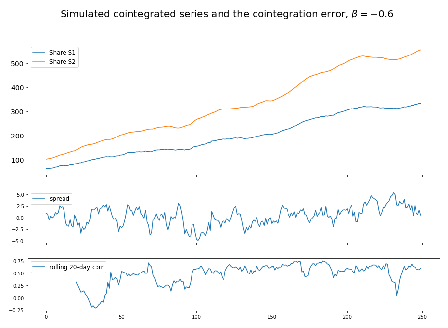
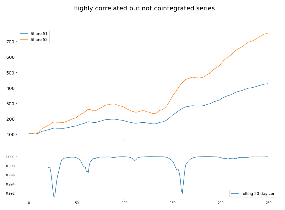
Figure 1 demonstrated an example of cointegrated series and the variation in its rolling 20-day correlation. Although the two asset price series are cointegrated and moving together, there exists a time period when the correlation between the returns of the two assets are negative. Figure 2 demonstrated an example of two highly correlated but not cointegrated series.

Figure 1. Cointegrated series can sometimes show negative correlation in returns.

Figure 2. Two highly correlated price series but not cointegrated at all. Engle-Granger test returned an ADF-statistics value of 0.41, which cannot reject the null hypothesis (two series not cointegrated) even at 90% significance.

Simulation of Cointegrated Series

Simulation is a powerful tool to understand a financial concept and cointegration is not an exception. The simulation of two cointegrated price series is now straightforward using the concepts introduced in the previous sections (Lin, 2006).

Returns are stationary. So we start with the simulation the returns of one asset using a stationary AR(1) process.
Retrieve the price by summing up the returns.
The spread between the two assets is stationary. Again, simulating this spread with a stationary AR(1) process.
Derive the price of the other asset using the cointegration relation.

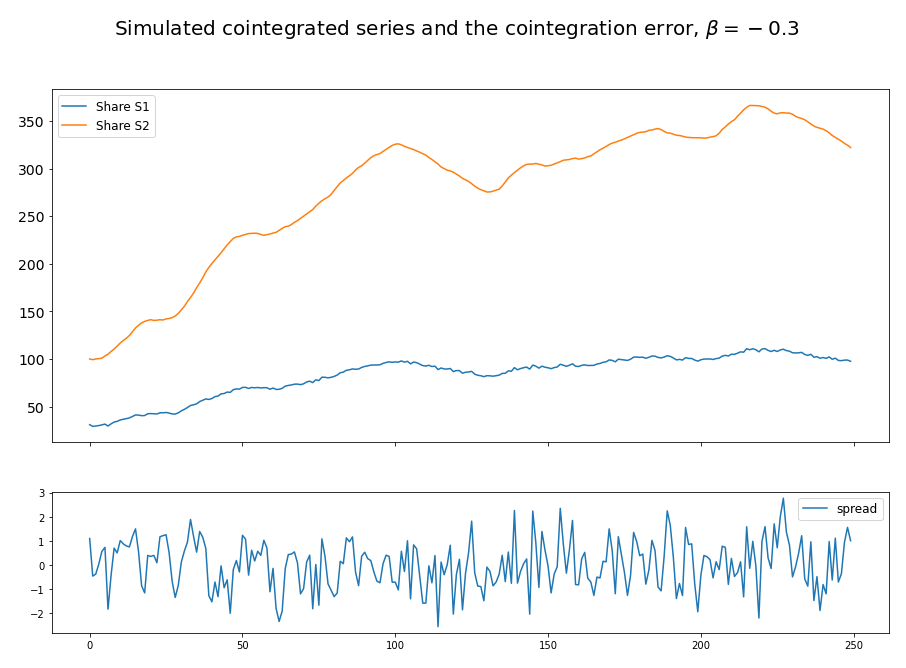
This is exactly how ArbitrageLab helps you simulate the prices of a pair of cointegrated assets. Figure 3 demonstrates the result of such a simulation.

Cointegrated series simulation ArbitrageLab

Figure 3. Cointegrated series simulation results from ArbitrageLab. The stationarity of the spread is demonstrated.

Derivation of the cointegration coefficient $\beta$

The two workhorses of finding the cointegration coefficient $\beta$ (or cointegration vector when there are more than 2 assets) are the Engle-Granger test (Engle, 1987) and the Johansen test. I will focus on the comparison of the two methods in terms of application rather than the mathematical underpinnings to prevent this article from getting into the quagmire of endless linear algebra. I will refer curious readers to (Johansen, 1988) and (Chan, 2013) for a more comprehensive introduction to Johansen test and Vector Error Correction Model (VECM).

Engle-Granger Test

The idea of Engle-Granger test is simple. We perform a linear regression between the two asset prices and check if the residual is stationary using the Augmented Dick-Fuller (ADF) test. If the residual is stationary, then the two asset prices are cointegrated. The cointegration coefficient is obtained as the coefficient of the regressor.

An immediate problem is in front of us. Which asset should we choose as the dependent variable? A feasible heuristic is that we run the linear regression twice using each asset as the dependent variable, respectively. The final $\beta$ would be the combination that yields a more significant ADF test.

But what if we have more than two assets? If we still apply the abovementioned heuristic, we will have to run multiple linear regressions, which is rather cumbersome. This is where Johansen test could come in handy.

Johansen Test

Johansen test uses the VECM to find the cointegration coefficient/vector $\beta$ . The most important improvement of Johansen Test compared to Engle-Granger test is that it treats every asset as an independent variable. Johansen test also provides two test statistics, eigenvalue statistics and trace statistics, to determine if the asset prices are statistically significantly cointegrated.

In conclusion, Johansen test is a more versatile method of finding the cointegration coefficient/vector $\beta$ than the Engle-Granger test. Both tests are implemented in ArbitrageLab, so finding the cointegration coefficient is no longer a problem.

A caveat: Raw prices or log prices?

Should we use raw prices or log prices in the cointegration tests? One key theme in this article is that prices are $I(1)$ series (which includes log-prices), and returns are $I(0)$ series. $I(0)$ series can be obtained by differencing the $I(1)$ series. So it comes naturally that log prices fit this description better, for the difference of log prices is directly log returns, but the difference of raw prices is not percentage returns yet. However, according to (Alexander, 2002), “Since it is normally the case that log prices will be cointegrated when the actual prices are cointegrated, it is standard, but not necessary, to perform the cointegration analysis on log prices.” So it is OK to analyze raw prices, but log prices are preferable.

Conclusion and Key Takeaways

Hopefully, this article helped you understand cointegration better. The key takeaways of this introductory are:

Cointegration describes a long-term relationship between asset prices.
Cointegration can be seen as a measure of similarity of assets in terms of risk exposure profiles.
The prices of cointegrated assets are tethered due to the stationarity of their spread.
Correlation and cointegration are two different concepts. Correlation is a short-term relationship between returns, while cointegration is a long-term relationship to prices. Do not use correlation for prices!
Engle-Granger and Johansen test can help find the cointegration coefficient/vector $\beta$ such that a cointegrated spread can be constructed.
ArbitrageLab can help with the simulation of cointegrated series and the calculation of $\beta$ .

Now that we know how to construct a stationary spread from a pair or even a group of assets, it is time to design a trading strategy that can take advantage of the stationarity of the spread. In Part 2 of this series, I will demonstrate two mean reversion pair/multi-asset trading strategies that can guarantee a minimum profit. Keep tuned.

Check out our lecture on the topic:

References

Footnote

https://www.nobelprize.org/prizes/economic-sciences/2003/summary/
Astute readers might have noticed that I did not give a rigorous definition of $I(0)$ series. In fact, the definition of $I(0)$ is not clear-cut. See When is a Time Series $I(0)$ ? for a discussion about the definition of $I(0)$ series.

References

- Alexander, C., Giblin, I. and Weddington, W., 2002. Cointegration and asset allocation: A new active hedge fund strategy. Research in International Business and Finance, 16 (5), pp.65-90.
- Chan, E., 2013. Algorithmic trading: winning strategies and their rationale (Vol. 625). John Wiley & Sons.
- Engle, R.F. and Granger, C.W., 1987. Co-integration and error correction: representation, estimation, and testing. Econometrica: Journal of the Econometric Society, pp.251-276.
- Galenko, A., Popova, E. and Popova, I., 2012. Trading in the presence of cointegration. The Journal of Alternative Investments, 15 (1), pp.85-97.
- Granger, C.W., 1981. Some properties of time series data and their use in econometric model specification. Journal of Econometrics, 16 (1), pp.121-130.
- Huck, N. and Afawubo, K., 2015. Pairs trading and selection methods: is cointegration superior?. Applied Economics, 47 (6), pp.599-613.
- Johansen, S., 1988. Statistical analysis of cointegration vectors. Journal of economic dynamics and control, 12 (2-3), pp.231-254.
- Lin, Y.X., McCrae, M. and Gulati, C., 2006. Loss protection in pairs trading through minimum profit bounds: A cointegration approach. Advances in Decision Sciences, 2006.
- McDermott, C.J., 1990. Cointegration: origins and significance for economists. New Zealand Economic Papers, 24 (1), pp.1-23.
- Stock, J.H. and Watson, M.W., 1988. Testing for common trends. Journal of the American statistical Association, 83 (404), pp.1097-1107.
- Vidyamurthy, G., 2004. Pairs Trading: quantitative methods and analysis (Vol. 217). John Wiley & Sons.