Bayesian Portfolio Optimisation: Introducing the Black-Litterman Model

By Aditya Vyas

Doing Meta-Analysis in R by Mathias Harrer et al.

Join the Reading Group and Community: Stay up to date with the latest developments in Financial Machine Learning!

The Black-Litterman (BL) model is one of the many successfully used portfolio allocation models out there. Developed by Fischer Black and Robert Litterman at Goldman Sachs, it combines Capital Asset Pricing Theory (CAPM) with Bayesian statistics and Markowitz’s modern portfolio theory (Mean-Variance Optimisation) to produce efficient estimates of the portfolio weights.

Before getting into the nitty-gritty of the algorithm it is important to understand the motivations behind developing it and why is it favored by practitioners in the industry. For a long while, investors worked under the assumption that the risk and return relationship of a portfolio was linear, meaning that if an investor wanted higher returns, they would have to take on a higher level of risk.

This assumption changed when in 1952, Harry Markowitz introduced Modern Portfolio Theory (MPT), which introduced the notion that the diversification of a portfolio can inherently decrease the risk of a portfolio. Simply put, this meant that investors could increase their returns while also reducing their risk. Markowitz’s work on MPT was groundbreaking in the world of asset allocation, eventually earning him a Nobel prize for his work in 1990.

However, investors soon encountered a major problem – even though it had a sound theory supporting it, MPT failed to produce favorable results in practice. The weights produced by the models did not match with the investors’ knowledge and failed to account for a lot of unexpected market variables. In short, after years of research, one can list down the following shortcomings of MPT:

High Input Sensitivity: MPT relies on the past performance of the market (returns and covariance matrix) to get an estimate of the portfolio holdings in the current market conditions. A big problem with this approach is that the performance of the past never provides a guarantee for the market situations that arise in the future. Small estimation errors in the past data leads to highly erroneous mean-variance portfolios.
Highly Concentrated Portfolios: The mean-variance procedure is found to be greedy and generates highly concentrated portfolios with only a few securities receiving the majority of allocations.
Neglecting Investor Knowledge: Finally, mean-variance optimization does not take into account an investor’s personal knowledge of the market conditions and intuition. In my opinion, this point can be considered to be the most important of the previously listed points. Rather than just relying on historical data, the models should also incorporate an investor’s own views of the market which is a very important asset. MVO, instead, chooses to use only historical data with a neglect for valuable market knowledge.

Reasons like the above and the underperformance of MPT in general enticed researchers to start looking for ways to improve it and come up with better models that can be used practically. The BL algorithm is one such model and although it has its own set of drawbacks, there are some unique features that make it an important part of a quant’s toolkit.

The rest of the article is structured as follows: In the first section, we explore an in-depth step-by-step understanding of the Black-Litterman algorithm. In the next section, we will see it in action by using PortfolioLab’s BL implementation and replicate the results of the original paper. This will be followed by a conclusion and references for further reading. You can click below on each item to go to the respective section.

Behind The Scenes: Into the Math of Black-Litterman
In Practice: Black-Litterman using PortfolioLab
Conclusion
References

Behind The Scenes: Into the Math of Black-Litterman

As mentioned previously, the Black-Litterman model relies heavily on Bayesian theory to generate its portfolios. We all know the classic Bayes formula equation:

$\begin{alignat*}{2} P(A|B) = \frac{P(A)P(B|A)}{P(B)} \end{alignat*}$

where, without going into much details, $P(A)$ is the prior distribution of $A$ , $P(B|A)$ is the likelihood distribution of $B$ given $A$ and $P(A|B)$ is the posterior distribution of $A$ . All 3 of these together – prior, likelihood, and posterior – make up a Bayesian model and this is exactly what makes up the Black-Litterman model too.

It has always been said that the Black-Litterman model is based on Bayesian theory but the literature on how it is exactly connected to the Bayes equation above is very sparse. In my opinion, it is much easier to get a hang of BL when it is broken down into the individual Bayesian elements of prior, likelihood, and posterior.

In this section, I will try to present it in a proper Bayesian framework with the appropriate derivations wherever necessary and hopefully, this will make it easier and more intuitive to understand.

The Prior: Implied Excess Equilibrium Returns

The model uses market equilibrium returns as the prior. But what exactly are these “equilibrium” returns? In simple words, they are the set of returns obtained by holding a CAPM market portfolio – one which theoretically contains all the assets in the universe. You will be familiar with the famous CAPM equation:

$\begin{alignat*}{2} E(r_i) = r_f + \beta_{i}(E(r_{market}) \: - \: r_f) \end{alignat*}$

where,

$r_f$ is the risk-free rate of return
$E(r_{market})$ is the expected rate of return of the market portfolio
$\beta_i$ is a market uncertainty variable which quantifies the variance in the return of the $i^{th}$ asset. It is given by $\beta_i = \frac{\sigma_{i, market}}{\sigma^{2}_{market}}$ where $\sigma_{i, market}$ is the covariance between the $i^{th}$ asset and market portfolio and $\sigma^{2}_{market}$ is the variance of the market portfolio.

Rearranging the above equation we get,

$\begin{alignat*}{2}\Pi &= \beta_{i}(E(r_{market}) \: - \: r_f)\end{alignat*}$

where, $\Pi$ is the excess equilibrium returns that we are interested in calculating. They are returns in excess of the risk-free market return.

The problem is how to find these returns? Fischer Black and Robert Litterman came up with a very cool trick to calculate them: reverse optimisation. Theoretically, in the CAPM universe all investors hold the market portfolio which contains every risky asset in the universe. Hence, one can use the market capitalisation of the assets for getting the appropriate weights allocations of the market portfolio.

$\begin{alignat*}{2}w^{i}_{market} = \frac{MC_{i}}{\sum_{j=1}^{N}MC_j}\end{alignat*}$

where $N$ is the number of assets in the portfolio and $MC_{i}$ is the market-cap of the $i^{th}$ asset.

Now, for any type of portfolio, an investor’s risk utility is given by the following equation:

$\begin{alignat*}{2}R \equiv w_{market}^{T}\Pi \: - \: \frac{\delta}{2}w^{T}_{alignat*}\Sigma w_{market}\end{alignat*}$

where,

$R$ is the risk utility.
$w_{market}$ is the vector of market portfolio weights – already calculated as discussed above.
$\Pi$ is the vector of excess equilibrium weights.
$\delta$ is the risk aversion parameter.
$\Sigma$ is the covariance matrix of asset returns.

The goal of any portfolio optimisation problem is to find the set of weights that minimise the risk-utlity for an investor. Now, the hessian of $R$ is given by:

$\begin{alignat*}{2}\frac{\partial^{2} R}{\partial w^{2}_{market}} = -\delta \Sigma < 0\end{alignat*}$

This quantity will be negative because $\Sigma$ is positive-definite which also leads to the $R$ being a concave function. Under no constraints, the risk utility will have a global maximum which will give us a least value of $R$ . We differentiate $R$ w.r.t $w$ and equate it to 0

$\begin{alignat*}{2}\frac{\partial R}{\partial w_{market}} = \Pi \: - \: \delta \Sigma w_{market} = 0\end{alignat*}$

$\begin{alignat*}{2}w_{market} = (\delta \Sigma)^{-1}\Pi\end{alignat*}$

Remember that we already have a way of calculating the market weights using the market-cap of the assets, which allows us to reverse the above equation and find the desired equilibrium returns

$\begin{alignat*}{2}\Pi = \delta \Sigma w_{market}\end{alignat*}$

This gives us our first distribution of the BL Bayesian model – $D_{prior}$

$\begin{alignat*}{2}\boxed{D_{prior} \equiv N(\Pi, \tau \Sigma)}\end{alignat*}$

where $\Pi$ and $\Sigma$ carry their usual meanings and $\tau$ is a constant of proportionality. The value of $\tau$ has been a source of great confusion among practitioners since the original paper also does not clarify its exact significance and what values does it take. I will not go into a lot of details and you will find a lot of papers and articles which explore its significance. It suffices to say that its value is always close to 0 and different papers use different values depending on the use-case.

The Likelihood: Market Views

The second step is to nail the likelihood distribution. In my opinion, this is one of the most important and ingenious aspects of the BL algorithm and you will soon see why. As we discussed earlier, one of the criticisms of the mean-variance theory was its inability to incorporate investor knowledge. This is important since it allows the weights to be influenced by the ever-changing market factors which an investor can observe and feed into the model.

For the purpose of this section, let us assume that we have a portfolio comprising of the following assets – Apple, Google, Microsoft, and Tesla – and we have some important market views about some of them. There are 3 main components that will allow investors to incorporate them into the model:

Views Vector: $Q$

The views vector contains information about the specific values pertaining to the market views. Let me explain this using an example. In the Black-Litterman world, there are two types of views:

Absolute Views: These are views that correspond to the scenario where an investor has assumptions on specific values of the market factors. Considering our example portfolio, let’s say we observe the current market conditions and develop the following views:
- Apple will yield a monthly expected return of 10%.
- Microsoft will only give a monthly return of 2%.
Relative Views: As the name suggests, these other type of views rely on relative performance comparisons between the portfolio assets. So, rather than specific estimates on the performance of Google and Tesla, we have the following view:
- Google will outperform Tesla (in terms of monthly expected returns) by 6%.

All of these views are then sent as input to the BL model through a $Kx1$ vector $Q$ , where $K$ refers to the number of views

Pick Matrix: $P$

With the view vector giving information about the specific view values, the pick matrix tells the model which assets from our portfolio are involved in each of these views. For $N$ assets in our portfolio, it is a $KxN$ matrix which looks like this:

Each row represents a view and the columns represent the assets in our portfolio. When only absolute views are involved, the asset involved in the view receives +1 while all others are 0. However, for relative views, the asset with better-expected performance (in our case Google) receives +1 while the other -1. This helps the model distinguish the outperforming assets from the underperforming ones. However, all this is well and good when there are at most 2 assets in our views, but what happens when there are more than 2 assets involved e.g. one might want to compare assets in one sector with those in another sector. Let’s say we also have the following view:

- Apple and Microsoft together will outperform Google and Tesla by 5%.

An obvious choice is to assign +1 to Apple-Microsoft, -1 to Google-Tesla, and then divide it equally among them. So, individually, Apple and Microsoft get +0.5 while Google and Tesla receive -0.5. The problem is there is no universally accepted method for specifying the pick values and different researchers have proposed different ways of doing so.

Litterman (2003, pg 82) uses a percentage value for the pick matrix while Satchell and Scowcroft (2000) employ an equal weighting scheme which is what I just described and also shown in the image above. However, I prefer the market-capitalization based assignment proposed in Idzorek (2004) – the weightings are assigned in proportion to the market-cap of the asset divided by the total market-cap of the sector/group. Based on this method, we get the following pick values: (I have considered the approximate market-cap of these assets at the time of writing)

$\begin{alignat*}{2}p_{AAPL} = \frac{MC_{AAPL}}{MC_{AAPL} + MC_{MSFT}} = 0.541\end{alignat*}$

$\begin{alignat*}{2}p_{MSFT} = \frac{MC_{MSFT}}{MC_{AAPL} + MC_{MSFT}} = 0.459\end{alignat*}$

$\begin{alignat*}{2}p_{GOOGL} = \frac{MC_{GOOGL}}{MC_{GOOGL} + MC_{TSLA}} = 0.745 \end{alignat*}$

$\begin{alignat*}{2}p_{TSLA} = \frac{MC_{TSLA}}{MC_{GOOGL} + MC_{TSLA}} = 0.255\end{alignat*}$

This is a better approach than the equal weighting scheme since it takes into account the relative importance of the assets within the outperforming and underperforming groups. So, even though the Apple-Microsoft group outperforms the other 2 assets, Apple with its larger market-cap has a more profound effect than Microsoft and the market-capitalisation based scheme helps the model capture this information.

Omega Matrix: $\Omega$

The final component is to take into account the error in investor judgment because, in the real world, no one can have market views with 100% confidence. Hence, a variance factor comes into play here which the model uses to adjust the final weights. Out of the 3 components discussed here – $Q$ , $P$ and $\Omega$ – the omega matrix can be considered the most important and also one of the most complex aspects of the BL model. It is a $KxK$ diagonal matrix where the diagonal values represent the variance in the corresponding views.

$\begin{alignat*}{2}\Omega= \left[ {\begin{array}{cccccc} \omega_1 & 0 & 0 & . & . & 0\\ 0 & \omega_2 & 0 & . & . & 0\\ 0 & 0 & . & . & . & 0\\ 0 & . & . & . & . & 0\\ 0 & . & . & . & . & 0\\ 0 & . & . & . & . & \omega_k\\ \end{array} } \right] \end{alignat*}$

Thus one can think of the investor’s expected return vector $E_{investor}(r)$ to be described by $Q$ and an error component $\epsilon$

$\begin{alignat*}{2} E_{investor}(r) & \sim Q \: + \: \epsilon \\ \epsilon & \sim \: N(0, \Omega) \end{alignat*}$

The error in views has 0 mean indicating no bias in an investor’s assumptions towards any particular assets in the portfolio. Another assumption is that all the error terms are uncorrelated and independent of each other – the reason for having a diagonal matrix.

Now an obvious question is how to create this matrix? Although the original paper does not give any details about a particular method, there has been a lot of research in this area and different papers have proposed varying ways of dealing with it. In this section, I will describe the most commonly used omega calculation method which was first proposed in He-Litterman (1999)

$\begin{alignat*}{2} \Omega = diag(P\tau \Sigma P^{T}) \end{alignat*}$

where, $diag()$ indicates creating a diagonal matrix from the diagonal elements of the target matrix and $\tau$ is a constant of proportionality whose values range from 0 to 1 (In the paper the authors use a $\tau = 0.05$ ). The assumption here is that the variance in the view errors will be proportional to prior variance and thus can be estimated only from the prior.

Combining all these components gives us our likelihood distribution $D_{likelihood}$

$\boxed{D_{likelihood} \equiv N(Q, \Omega)}$

The BL posterior portfolio always oscillates between two extremes – one scenario where the investor has 100% confidence in the views ( $\Omega = 0$ ) and the other where he/she has no confidence in the specified views ( $\Omega = \inf$ ).

When the investor has zero confidence in their views, the prior distribution dominates, and the posterior portfolio is shifted towards the prior. On the other hand, when the views are specified with 100% confidence, the posterior distribution of the parameters is dominated by only the views, neglecting any prior knowledge.

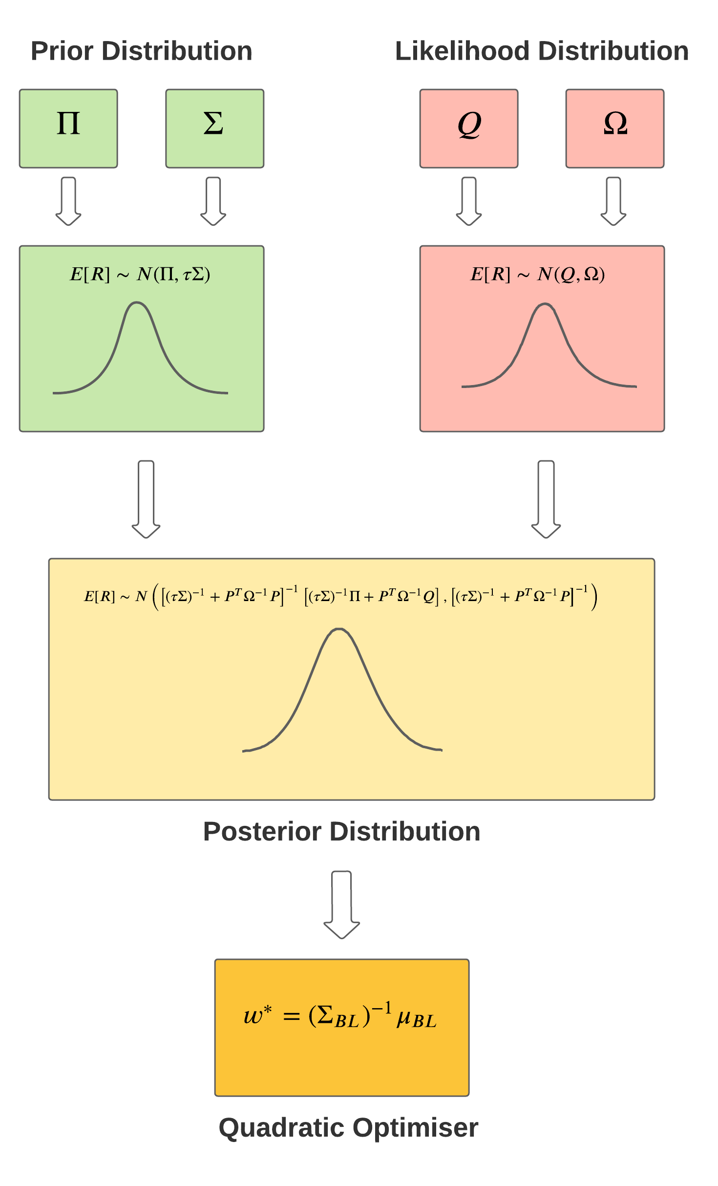
The Posterior: The Master Formula

Combining both the prior and likelihood gives us the following Black-Litterman posterior distribution

$\begin{equation*} \boxed{ \begin{alignat*}{2} D_{BL} & \equiv N(\mu_{BL}, \Sigma_{BL}) \\ \mu_{BL} & = ((\tau \Sigma)^{-1} + P^{T}\Omega^{-1}P)^{-1}((\tau \Sigma)^{-1}\Pi + P^{T}\Omega^{-1}Q) \\ \Sigma_{BL} & = ((\tau \Sigma)^{-1} + P^{T}\Omega^{-1}P)^{-1} \end{alignat*} } \end{equation*}$

The above set of formulae for the mean and covariance is known as the Master Formula. It looks quite complex but the calculation of the equations is a simple application of the Bayes Rule. In this section I will be going into the details of its derivation and it will involve some math, so feel free to skip over to the next section if you want.

In the Black-Litterman world, the first assumption is that market returns $R$ are normally distributed with a true hidden mean $\mu$ and covariance $\Sigma$ .

$\begin{alignat*}{2}R \sim N(\mu, \Sigma)\end{alignat*}$

Ofcourse, these true hidden parameters can never be known with certainty but we can always try to predict their underlying distribution and ultimately the distribution of returns. With respect to this, let us treat the mean as a random variable $\textbf{E(r)}$ . This gives us the following two assumptions:

Without any constraints, the prior distribution acts as the sampling distribution for $\textbf{E(r)}$

$\textbf{E(r)} \sim D_{prior} \equiv N(\Pi, \tau \Sigma)$

Conditioned upon the prior, one can get sample mean vectors from the likelihood distribution.

$\begin{alignat*}{2}\textbf{PE(r)} \: | \: \textbf{E(r)} \sim D_{likelihood} \equiv N(Q, \Omega)\end{alignat*}$

Note that $P$ here refers to the pick matrix and acts as an indexing matrix to select those assets of $\textbf{E(r)}$ for which the investor has views.

For a specific mean vector $e(r)$ sampled from $\textbf{E(r)}$ , the probability density functions of prior and likelihood are a direct application of the pdf of multivariate normal distribution:

$\begin{alignat*}{2} f_{\textbf{E(r)}}(e(r)) = \frac{|\tau \Sigma|^{-1/2}}{(2\pi)^{N/2}}exp(-\frac{1}{2}(e(r) - \Pi)^{T}(\tau \Sigma)^{-1}(e(r) - \Pi)) \end{alignat*}$

$\begin{alignat*}{2} f_{\textbf{PE(r)}|\textbf{E(r)}}(Pe(r)) = \frac{|\Omega|^{-1/2}}{(2\pi)^{N/2}}exp(-\frac{1}{2}(Pe(r) - Q)^{T}(\Omega)^{-1}(Pe(r) - Q)) \end{alignat*}$

The posterior distribution $\textbf{E(r)} \: | \: \textbf{PE(r)}$ can be calculated using the Bayes Rule. The equation needs to be reformatted so that the left hand side is proportional to a conditiona pdf $f_{\textbf{E(r)}|\textbf{PE(r)}}$ times a factor. The conditional aspect of the equation will be the required pdf and will give us the values for the posterior mean and covariance.

$\begin{alignat*}{3} f_{\textbf{E(r)}|\textbf{PE(r)}}(e(r)) &= \frac{f_{\textbf{E(r)}}(e(r))f_{\textbf{PE(r)}|\textbf{E(r)}}(Pe(r))}{f_{\textbf{PE(r)}}(Pe(r))} \\[5pt] &= \frac{f_{\textbf{E(r)}}(e(r))f_{\textbf{PE(r)}|\textbf{E(r)}}(Pe(r))}{\bigintss f_{\textbf{E(r)}}(e^{'}(r))f_{\textbf{PE(r)}|\textbf{E(r)}}(Pe^{'}(r))\:de^{'}(r)} \\[5pt] &\propto exp(-\frac{1}{2}((e(r) - \Pi)^{T}(\tau \Sigma)^{-1}(e(r) - \Pi) + (Pe(r) - Q)^{T}(\Omega)^{-1}(Pe(r) - Q))) \end{alignat*}$

All the other terms – $(2\pi)^{-N/2}$ , $|\tau \Sigma|^{-1/2}$ , $|\Omega|^{-1/2}$ and the integral denominator – do not contribute to the final conditional pdf terms and can be ignored as as a proportionality factor. Let us focus on the term within the exponential and break it down to get the desired form.

$\begin{alignat*}{2} f_{\textbf{E(r)}|\textbf{PE(r)}}(e(r)) &\propto exp(\frac{-1}{2}(e(r)^{T}(\tau \Sigma)^{-1}e(r) - e(r)^{T}(\tau \Sigma)^{-1}\Pi - \Pi^{T}(\tau \Sigma)^{-1}e(r) + \Pi^{T}(\tau \Sigma)^{-1}\Pi \\ & \qquad + e(r)^{T}P^{T}\Omega^{-1}Pe(r) - e(r)^{T}P^{T}\Omega^{-1}Q - Q^{T}\Omega^{-1}Pe(r) + Q^{T}\Omega^{-1}Q)) \end{alignat*}$

Notice that $e(r)^{T}(\tau \Sigma)^{-1}\Pi$ is symmetric with $\Pi^{T}(\tau \Sigma)^{-1}e(r)$ and $e(r)^{T}P^{T}\Omega^{-1}Q$ is symmetric with $Q^{T}\Omega^{-1}Pe(r)$ . We can combine them together to simplify the equation further,

$\begin{alignat*}{3} f_{\textbf{E(r)}|\textbf{PE(r)}}(e(r)) & \propto exp(-\frac{1}{2}(e(r)^{T}(\tau \Sigma)^{-1}e(r) - 2\Pi^{T}(\tau \Sigma)^{-1}e(r) + \Pi^{T}(\tau \Sigma)^{-1}\Pi \\ & \qquad + e(r)^{T}P^{T}\Omega^{-1}Pe(r) - 2Q^{T}\Omega^{-1}Pe(r) + Q^{T}\Omega^{-1}Q)) \\[5pt] & \propto exp(-\frac{1}{2}( e(r)^{T}\left[(\tau\Sigma)^{-1} + P^{T}\Omega^{-1}P\right]e(r) - 2\left[\Pi^{T}(\tau\Sigma)^{-1} + Q^{T}\Omega^{-1}P\right]e(r)\\ & \qquad + \Pi^{T}(\tau \Sigma)^{-1}\Pi + Q^{T}\Omega^{-1}Q)) \\ \end{alignat*}$

To make it easy to follow the steps, let us make the following substitutions

$\begin{alignat*}{2} A &= (\tau\Sigma)^{-1}\Pi + P^{T}\Omega^{-1}Q \\ B &= (\tau\Sigma)^{-1} + P^{T}\Omega^{-1}P \\ C &= Q^{T}\Omega^{-1}Q + \Pi^{T}(\tau\Sigma)^{-1}\Pi \end{alignat*}$

Continuing from where we left off,

$\begin{alignat*}{2} f_{\textbf{E(r)}|\textbf{PE(r)}}(e(r)) &\propto exp(-\frac{1}{2}( e(r)^{T}Be(r) - 2A^{T}e(r) + C )) \\ \end{alignat*}$

We make use of the following facts: $B$ is symmetric with $B = B^{T}$ and $B^{-1}B = I$ , where $I$ is the identity matrix.

$\begin{alignat*}{3} & \propto exp(-\frac{1}{2}((Be(r))^{T}B^{-1}Be(r) - 2A^{T}B^{-1}Be(r) + C)) \\ & \propto exp(-\frac{1}{2}((Be(r))^{T}B^{-1}Be(r) - 2A^{T}B^{-1}Be(r) + C - A^{T}B^{-1}A + A^{T}B^{-1}A)) \\ & \propto exp(-\frac{1}{2}((Be(r) - A)^{T}B^{-1}(Be(r) - A) + C - A^{T}B^{-1}A)) \\ & \propto exp(-\frac{1}{2}((e(r) - B^{-1}A)^{T}B(e(r) - B^{-1}A) + C - A^{T}B^{-1}A)) \\ & \propto exp(-\frac{1}{2}((e(r) - B^{-1}A)^{T}B(e(r) - B^{-1}A))exp(-\frac{1}{2}(C - A^{T}B^{-1}A)) \\ f_{\textbf{E(r)}|\textbf{PE(r)}}(e(r)) & \propto exp(-\frac{1}{2}((e(r) - B^{-1}A)^{T}B(e(r) - B^{-1}A)) \end{alignat*}$

If we compare the above result with the pdf equation for a multivariate normal distribution, then the mean and covariance reveal themselves

$\begin{alignat*}{2} \mu &= B^{-1}A = ((\tau\Sigma)^{-1} + P^{T}\Omega^{-1}P)^{-1}((\tau\Sigma)^{-1}\Pi + P^{T}\Omega^{-1}Q) \\ \Sigma &= B^{-1} = ((\tau\Sigma)^{-1} + P^{T}\Omega^{-1}P)^{-1} \end{alignat*}$

Optimal Portfolio Weights

The final weights can be found by simply plugging the posterior mean and covariance into a standard mean-variance solver. Under no constraints, the following equation holds true.

$\begin{alignat*}{2} w^{*} = (\Sigma_{BL})^{-1}\mu_{BL} \end{alignat*}$

Note that the new mean and covariance can be passed into any custom optimisation problem and the above equation is true only for a no constraints problem.

This completes the working of the Black-Litterman algorithm. You can see that the views and prior distributions play a very important role in how the final BL portfolio is formed. The following graphic represents the Black-Litterman model in its entirety.

In Practice: Black-Litterman using PortfolioLab

Now that we have looked at the underlying theory of the BL model, let us run it on real-world financial data. The Black-Litterman model is available in the portfolio optimisation module of PortfolioLab. It is the latest offering from Hudson and Thames – a library dedicated for portfolio optimisation. You can install it from PyPi

pip install portfoliolab

Next up we import the Black-Litterman implementation:

from portfoliolab.bayesian import VanillaBlackLitterman

We will be using the model to replicate results from the He-Litterman paper – The Intuition Behind Black-Litterman Model Portfolios. In this paper, the authors test the BL algorithm on a market consisting of equity indexes of seven major industrial countries. It is a small dataset but helps to understand the working of the model clearly.

countries = ['AU', 'CA', 'FR', 'DE', 'JP', 'UK', 'US']

# Table 1 of the He-Litterman paper: Correlation matrix
correlation = pd.DataFrame([
    [1.000, 0.488, 0.478, 0.515, 0.439, 0.512, 0.491],
    [0.488, 1.000, 0.664, 0.655, 0.310, 0.608, 0.779],
    [0.478, 0.664, 1.000, 0.861, 0.355, 0.783, 0.668],
    [0.515, 0.655, 0.861, 1.000, 0.354, 0.777, 0.653],
    [0.439, 0.310, 0.355, 0.354, 1.000, 0.405, 0.306],
    [0.512, 0.608, 0.783, 0.777, 0.405, 1.000, 0.652],
    [0.491, 0.779, 0.668, 0.653, 0.306, 0.652, 1.000]
], index=countries, columns=countries)

# Table 2 of the He-Litterman paper: Volatilities
volatilities = pd.DataFrame([0.160, 0.203, 0.248, 0.271, 0.210, 0.200, 0.187],
                            index=countries, columns=["vol"])
covariance = volatilities.dot(volatilities.T) * correlation

The market equilibrium weights are calculated using the market-cap of the indices.

# Table 2 of the He-Litterman paper: Market-capitalised weights
market_weights = pd.DataFrame([0.016, 0.022, 0.052, 0.055, 0.116, 0.124, 0.615],
                              index=countries, columns=["CapWeight"])

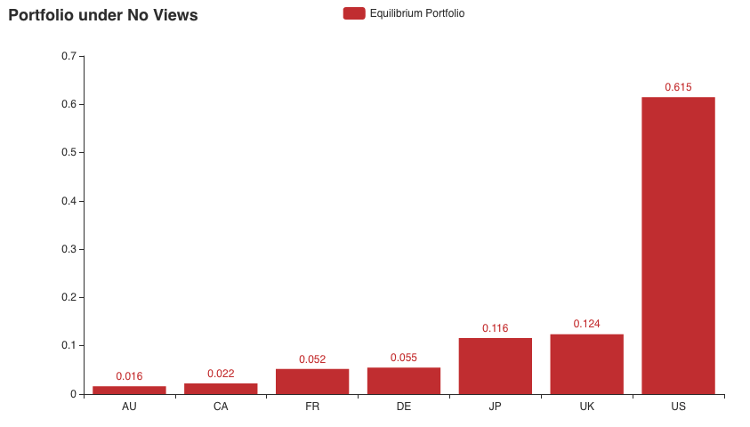
Under no market views, the investor holds the market portfolio shown above. Now let us start introducing some views.

View-1: Germany vs Rest of Europe

The first view explored by the authors states that German equities will outperform the rest of the European equities by 5%. We have one German equity in our portfolio – DE – and two European equities – FR and UK. We create the views vector and the pick list:

# Q
views = [0.05]

# P
pick_list = [
        {
            "DE": 1.0,
            "FR": -market_weights.loc["FR"]/(market_weights.loc["FR"] + \
                                            market_weights.loc["UK"]),
            "UK": -market_weights.loc["UK"] / (market_weights.loc["FR"] + \
                                                market_weights.loc["UK"])
        }
]

The pick list parameter in VanillaBlackLitterman class expects list of dictionaries specifying the assets participating in each view and the corresponding pick values. Internally, the code will convert this representation to the pick matrix $P$ mentioned previously. Here we are using the capitalisation of the assets to calculate the respective pick values.

Finally it is time to allocate weights using the allocate() method.

bl = VanillaBlackLitterman()
bl.allocate(covariance=covariance,
            market_capitalised_weights=market_weights,
            investor_views=views,
            pick_list=pick_list,
            asset_names=covariance.columns,
            tau=0.05,
            risk_aversion=2.5)

You can access the final results using four main class variables – implied_equilibrium_weights, posterior_expected_returns, posterior_covariance and weights.

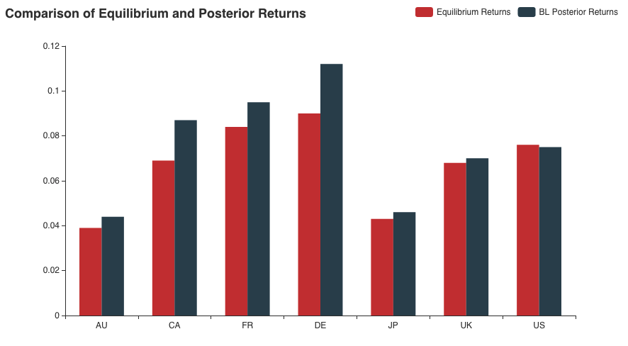
Let’s look at a comparison between the equilibrium and BL posterior returns for View-1

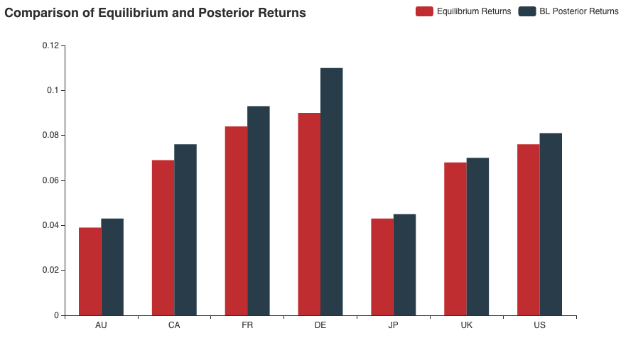
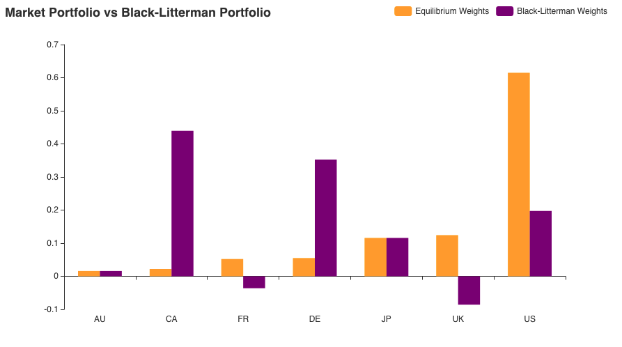
One can notice that based on the positive view specified, the model has increased the returns of German equity relative to the others. However, note that since the market portfolio already had slightly higher returns for DE as compared to FR and UK, the relative increase due to the view is not so significant. The weight distribution, however, tells a different story.

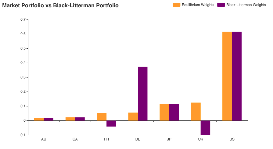
Literally, all assets not involved in the view have their weights unchanged. On the other hand, the BL model increased the allocations for DE and made the weights of European equities negative! It is straight up telling us to short these assets. You can observe how a small view of 5% had such a visible effect on our portfolio. Now let us complicate this further by adding some more views.

View-2: Canada vs US

For this view, the investor thinks that Canadian equities will outperform US equity by 3% annually.

# Q
views = [0.05, 0.03]

# P
pick_list = [
    {
        "DE": 1.0,
        "FR": -market_weights.loc["FR"]/(market_weights.loc["FR"] + market_weights.loc["UK"]),
        "UK": -market_weights.loc["UK"] / (market_weights.loc["FR"] + market_weights.loc["UK"])
    },
    {
        "CA": 1,
        "US": -1
    }
]

# Allocate
bl = VanillaBlackLitterman()
bl.allocate(covariance=covariance,
            market_capitalised_weights=market_weights,
            investor_views=views,
            pick_list=pick_list,
            asset_names=covariance.columns,
            tau=0.05,
            risk_aversion=2.5)

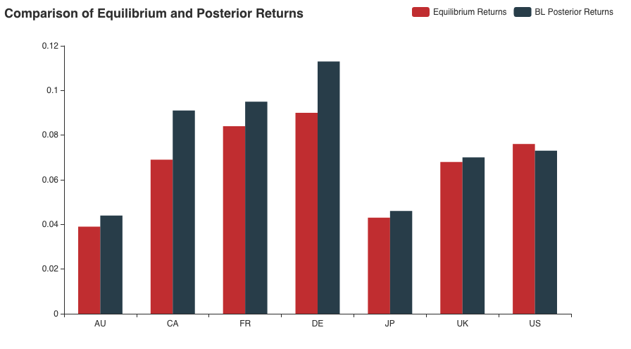
Note that we are also keeping the first view and adding a layer of complexity by introducing View-2. Let us see how our final portfolio looks like.

The result above is intuitively very easy to understand. The annualized returns on Canadian equities have increased further while those for the US have gone down a bit. Returns for DE, FR, and UK stay in conjunction with the first view. However, the most visible change can be seen in the weight distribution of the portfolio. Canadian equities see a 95% increase in the allocation while that of the US gets reduced by almost 67%. The German and European equities’ allocations remains unaffected.

View-3: More Bullish Canada vs the US

As the last example, the authors decide to make View-2 more bullish. Instead of a 3% return, the investor now expects CA to outperform the US by 4%.

# Q
views = [0.05, 0.04]

# P
pick_list = [
    {
        "DE": 1.0,
        "FR": -market_weights.loc["FR"]/(market_weights.loc["FR"] + market_weights.loc["UK"]),
        "UK": -market_weights.loc["UK"] / (market_weights.loc["FR"] + market_weights.loc["UK"])
    },
    {
        "CA": 1,
        "US": -1
    }
]

# Allocate
bl = VanillaBlackLitterman()
bl.allocate(covariance=covariance,
            market_capitalised_weights=market_weights,
            investor_views=views,
            pick_list=pick_list,
            asset_names=covariance.columns,
            tau=0.05,
            risk_aversion=2.5)

Note that the $P$ does not change here since we are only changing the view value.

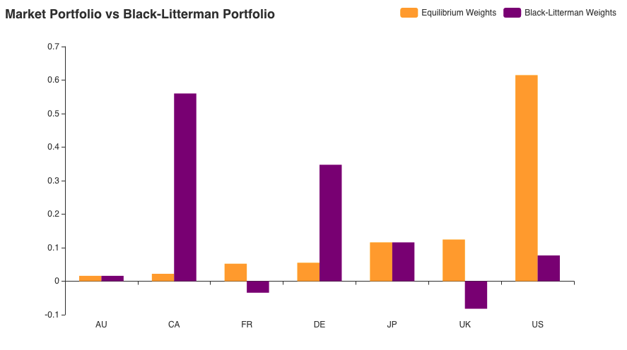
The returns remain almost unchanged w.r.t View-2 return distribution. However, one can observe that a more bullish view on CA has led the BL model to increase its overall portfolio allocation to 56%! And correspondingly, the US allocations have been reduced to a meager 7% of the total holdings.

Conclusion

This article explores the intuition, mathematical formulations, and the practical uses of the Black-Litterman model, which is regarded by many as an important portfolio allocation algorithm developed in its time. Despite all the complexity, it is a simple application of the Bayes Rule and by formulating the model in the form of prior, likelihood, and posterior distributions, the working and intuition behind the steps becomes much easier to understand.

In my opinion, one of the main reasons BL works so nicely is that it helps investors and analysts incorporate their own beliefs and views of the market – something which is ever-changing with the market conditions. This creates a model that is robust and less sensitive to the changing market dynamics and at the same time also handles variance in these views efficiently.

However, not everything is foolproof and the Black-Litterman model does suffer from some limitations:

Assumption of normality – At the end of the day, even Black-Litterman could not escape the simplicity of normal assumption of the market returns. Assuming a normal distribution for the returns makes the model constrained and not entirely flexible to adapt to the true market parameters.
Views constrained to returns – As mentioned previously, the ability to allow investors to specify their own views is one of the most noteworthy characteristics of the BL model. However, it is only really constrained to views on expected returns. The model can really be improved by allowing views on diverse market parameters like correlations, covariances, and variance between the returns, etc…
Limitations of the market portfolio – The equilibrium portfolio plays an important role in the BL model. Hence, any changes in the market portfolio will affect the final posterior BL weights. The problem is that the practicality the market portfolio is very hard to define. There are many risky assets trading in the world but they do not represent the entirety of the market securities. As a result, although in theory one can hold an equilibrium portfolio, in the practical world, it is very easy to get less than optimal BL allocations because of an improper market portfolio.
Sensitivity to investor inputs – Although all portfolio optimisation models suffer from sensitivity to input data, BL is affected more so because of the added parameter of investor beliefs. As you saw in the bullish view of Canada vs the US, increasing the belief by just 1% led to such a dramatic change in the final portfolio allocations. Thus, one needs to be extra careful when trying to input their views as they can sway the final allocations in either direction very easily.

References

- Black, F. and Litterman, R., 1990. Asset allocation: combining investor views with market equilibrium. Goldman Sachs Fixed Income Research, 115.
- Tetyana Polovenko, 2017. Black-Litterman Model
- Idzorek, T., 2007. A step-by-step guide to the Black-Litterman model: Incorporating user-specified confidence levels. In Forecasting expected returns in the financial markets (pp. 17-38). Academic Press.
- Meucci, A., 2006. Beyond Black-Litterman in practice: A five-step recipe to input views on non-normal markets. Available at SSRN 872577.
- Walters, C.F.A., 2014. The Black-Litterman model in detail. Available at SSRN 1314585.
- Narrow Margin, 2012. The Parameter Tau in Idzorek’s Version of the Black-Litterman Model
- He, G. and Litterman, R., 2002. The intuition behind Black-Litterman model portfolios. Available at SSRN 334304.