Copula for Statistical Arbitrage: Stocks Selection Methods
by Hansen Pei, Vijay Nadimpalli
Join the Reading Group and Community: Stay up to date with the latest developments in Financial Machine Learning!
This is the fifth article of the copula-based statistical arbitrage series. You can read the previous four articles with the first three focusing on pairs-trading:
LEARN MORE ABOUT PAIRS TRADING STRATEGIES WITH “THE DEFINITIVE GUIDE TO PAIRS TRADING”
Introduction
Copula is a very flexible tool for modeling dependencies among random variables. Long been used in risk management, it is also a great statistical arbitrage method when coupled with a good execution rule that is not limited to just mean-reversion strategies. From 2010, multiple trading methods involving copula have been developed: from earlier simple bi-variate copula on prices series to recent sophisticated self-adaptive models using low-latency data. It is a growing and dynamic field of research and practice, however, there is little literature reviewing criteria for selecting tradable stocks dedicated solely to copula-based methods.
[Rad et al (2016)] found that the copula pairs-trading method (the version that they implemented) has much better performance in drawdown risk compared to distance and cointegration, however, bad pairs that fail to converge significantly drove down its performance. It is a serious reminder to practitioners that building a suitable portfolio is just (if not more) as important as applying a great trading method, and a less desirable set of securities can quickly ruin a seemingly great strategy. The Vine copula is created to model across multiple random variables and therefore poses a greater challenge in selecting stocks.
In this article, we aim to introduce several stocks-selection methods popular for copula strategies, especially one proposed by [Mangold (2016)] that uses copula itself to form partners with a focus on representing extreme tail co-moves.
Why Stocks Selection is Difficult
Say that we found a way to generate trading signals using copula, then selecting stocks for this method can somewhat be considered its dual problem (in the operator space): given this copula method, which way is the “best” to maximize the profit on average. Mathematically this is already a very challenging problem given the nature of copula, and practically one also at least cares about risk, the abundance of tradable opportunities, and trading frequencies.
Moreover, copula is an extremely flexible method, and any other method that can deal with financial time series can be coupled with copula: Copula itself does not generate tradable signals. The key value it calculates is the conditional probability that is difficult to estimate empirically. Say there are 3 stocks ![]() , copula calculates (Note: those values are model dependent)
, copula calculates (Note: those values are model dependent)
(1) 
or the demeaned cumulative sum of their returns conditional probabilities (Also called CMPI for cumulative mispricing index. I know this is a long sentence and it may not make any sense to you at the moment. But I promise it is not bad if you read through Copula for Pairs Trading: A Unified Overview of Common Strategies.)
Those conditional probability (or CMPI) series capture the relative mispricing of the random variables. If you plot them, they look quite similar to the prices series themselves. Therefore what copula does is the following, and nothing more than it:
It essentially processes financial time series into another set of time series that reflects relative mispricing of stocks. And the processed series visually looks like the original prices series.
We immediately have the following:
- Any strategy that handles price time series can be used in combination with copula.
- Suppose each of such methods has one optimal corresponding stocks selection criterion, there is overall no optimal stocks selection criterion for all methods that involve copula.
And as a result:
Stocks selection methods should be curated to the trading strategy. There are no global selection methods that outperform all others.
For example, a mean-reverting bet will select different stocks compared to a quality minus junk bet. Since most people focus on mean-reverting strategies and those are what we have implemented in ArbitrageLab, we will focus on stock selection methods with that in mind. In general, we want to find methods that are:
- Use rank statistics.
- Fast to compute.
- Related to forming a mean-reverting portfolio.
- Take advantage of copula’s ability in modeling tail co-moves.
Conventional Methods
Conventional methods are often used widely in practice due to their interpretability and ease of implementation, though they may not satisfy all of our requirements above. Often they are already implemented in other packages and can be quickly adapted. We list a few representative methods with different areas of focus. Since those are in general quite common, we won’t spend much time here to introduce them from scratch. All methods mentioned are available in ArbitrageLab unless stated otherwise.
Bivariate
- Euclidean distance on prices or returns.
- Pearson’s correlation on prices or returns. Note that this value only captures linear correlation.
- Spearman’s
 and Kendall’s
  on prices or returns. Those two yield very similar candidates with Kendall’s
  being computationally heavier but slightly more stable. Also, a less-known fact is that the two statistics detect the monotonic relationship: it does not have to be that the two stocks must move together in the same direction to be detected, it can be that one goes down when another goes up.
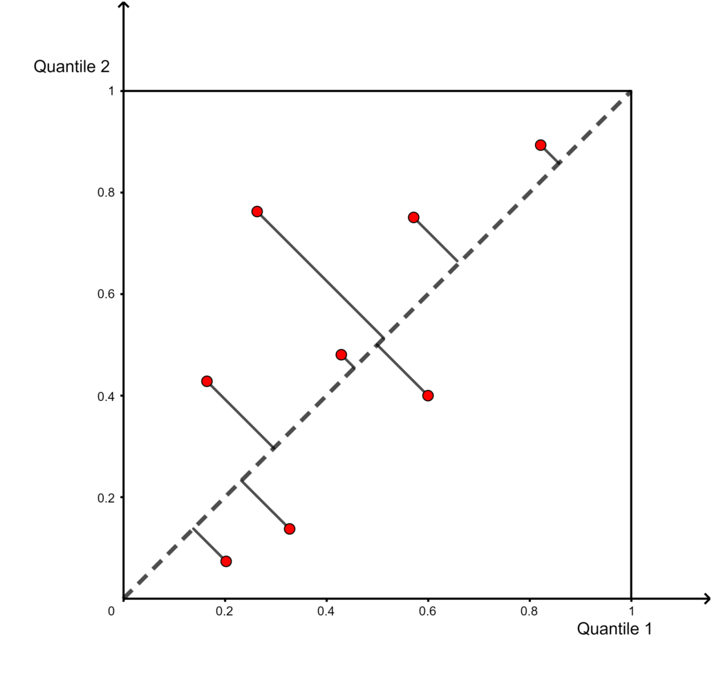
 - Quantile-Quantile plot’s averaged diagonal distance. The smaller the distance the more “related” they are (in one direction). This can be considered a statistic for the empirical copula.
- Test whether the two distributions are the same: Van der Waerden test on returns, a non-parametric test statistic to determine if the two distributions follow the same distribution. The main advantage is that it is robust even when the underlying normality assumption is not satisfied [Lüpsen (2016)]. Available in scikit-posthocs.
- Test for cointegration: Engle-Granger, Johansen etc.
- Test the stationarity of time series: One can use, for example, Hurst exponent for a spread between the two time series.
Fig 1: Illustration of the averaged diagonal distance method.
Multivariate
[Stübinger et al (2018)] proposes a multivariate vine copula-based statistical arbitrage framework, where specifically, for each stock in the S&P 500 database, the three most suitable partners are selected by leveraging different selection criteria.
We focus on the four multivariate partner selection approaches implemented in arbitragelab, as described in the paper. These partner selection approaches include the three multivariate approaches and a standout copula-based approach.
Before we move on to demonstrating these approaches, here are some important things to consider.
Firstly, all measures of association are calculated using the ranks of the daily discrete returns of our samples. Ranked transformations are preferred as copulas deal primarily with ranked statistics, and because ranked data provides robustness against outliers since we only consider the relative position of outliers in the ordered sample instead of the value of itself.
Secondly, the stock for which partners are selected is called a target stock. These selected partners for a target stock are called partner stocks.
The traditional, the extended, and the geometric approach share a common feature – they measure the deviation from linearity in ranks. Put simply, these methods measure how linearly related these ranks are with each other using a quantitative formula. All three approaches aim at finding the quadruple that behaves as linearly as possible to ensure that there is an actual relation among its components to model. These approaches also rule out nonlinear dependencies in ranks.
On the other hand, the copula based extremal approach tries to maximize the distance to independence with a focus on the joint extreme observations. This aspect makes this approach work well for the C-Vine copula mean-reversion strategies we implemented because copulas are great at handling extremities.
Importing the module
from arbitragelab.copula_approach.vine_copula_partner_selection import PartnerSelection
from arbitragelab.copula_approach.vine_copula_partner_selection_utils import get_sector_data
import pandas as pd
Loading the dataset
We use a dataset containing daily pricing data of all stocks in S&P 500 from the year 2019.
# Importing DataFrame of daily pricing data for all stocks in S&P 500.(at least 12 months data)
df = pd.read_csv('./sp500_2019.csv', parse_dates=True, index_col='Date').dropna()

# Instantiating the partner selection module.
ps = PartnerSelection(df)

#Loading the sector data for every stock in S&P 500
constituents = pd.read_csv('./sp500_constituents-detailed.csv', index_col='Symbol')
1. Pairwise Spearman’s  .
.
As a baseline approach, the high dimensional relation between the four stocks is represented by their pairwise Spearman’s ![]() . The use of ranked returns data allows us to capture non-linearities in the data to a certain degree.
. The use of ranked returns data allows us to capture non-linearities in the data to a certain degree.
The procedure is as follows:
- For each target stock, calculate the sum of all pairwise Spearman’s
 , for all possible quadruples consisting of the fixed target stock.
 - Return the final quadruple with the largest sum of pairwise Spearman’s
 for each target stock.
# Calculating final quadruples using the traditional approach for the first 10 target stocks.
traditional_Q = ps.traditional(10)

print(pd.Series(traditional_Q))
Output:
0         [A, TMO, PKI, MTD]
1       [AAL, UAL, LUV, DAL]
2    [AAP, AMAT, KLAC, LRCX]
3    [AAPL, MCHP, TXN, MXIM]
4        [ABBV, A, TMO, PKI]
5       [ABC, MCK, CAH, WBA]
6     [ABMD, ISRG, ABT, BSX]
7         [ABT, DHR, TMO, A]
8         [ACN, MA, V, PYPL]
9        [ADBE, MA, V, PYPL]
2. Multivariate Spearman’s  .
.
[Schmid and Schmidt (2007)] introduced a multivariate rank based measures of association. This paper generalizes Spearman’s ![]() to arbitrary dimensions – a natural extension of the baseline approach.
to arbitrary dimensions – a natural extension of the baseline approach.
In contrast to the strictly bi-variate case, this extended approach – and the two following approaches – directly reflect multivariate dependence instead of measuring it by pairwise measures only. This approach provides a more precise modeling of high dimensional association and thus we expect a better performance in trading strategies compared to the baseline traditional approach.
Given below is a brief overview of the methodology used in [Schmid and Schmidt (2007)] to calculate the multivariate Spearman’s ![]() .
.
We let ![]() denote the number of stocks for which daily returns are observed from day
denote the number of stocks for which daily returns are observed from day ![]() to day
to day ![]() .
. ![]() denotes the
denotes the ![]() -th stock’s daily return.
-th stock’s daily return.
- We use
 to calculate the quantile data from returns for stock
  .
.
(2) ![]()
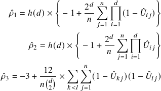
The authors proposed three generalized formulas for the Spearman’s ![]() in a higher dimension, with a focus on different technical aspects that we will not get into here. These three formulas all boils down to the Spearman’s
in a higher dimension, with a focus on different technical aspects that we will not get into here. These three formulas all boils down to the Spearman’s ![]() when
when ![]() . For our implementation, we take the average of the three as our final measure:
. For our implementation, we take the average of the three as our final measure:
(3) 
Where:
(4) ![]()
The procedure is as follows:
- For each target stock, calculate the mean of the three generalized formulas for Spearman’s
 , for all possible quadruples consisting of a fixed target stock.
 - Quadruple with the largest value is considered as the final quadruple for each target stock.
# Calculating final quadruples using the extended approach for the first 10 target stocks.
extended_Q = ps.extended(10)
print(pd.Series(extended_Q))
Output:
Please note that in the output below, the first ticker in the respective lists is the target stock.
0         [A, TMO, PKI, MTD]
1       [AAL, UAL, LUV, DAL]
2    [AAP, AMAT, KLAC, LRCX]
3    [AAPL, MCHP, TXN, MXIM]
4        [ABBV, A, TMO, PKI]
5       [ABC, MCK, CAH, WBA]
6     [ABMD, ISRG, ABT, BSX]
7         [ABT, DHR, TMO, A]
8         [ACN, MA, V, PYPL]
9        [ADBE, MA, V, PYPL]
3. Quantile plot’s hyper-diagonal distance.
This approach measures a geometric relationship between the stocks in the quadruple. It involves calculating the sum of euclidean distances from the 4-dimensional hyper-diagonal in their quantile plots.
To explain this technique briefly, let’s consider the relative ranks(quantiles) of a bi-variate random sample, where every observation takes on values in the ![]() square. The diagonal line in this square represents a perfectly linear relationship between the ranks of the components of the sample. However, if this relationship is not perfectly linear, at least one point differs from the diagonal. The sum of euclidean distances of all ranks from the diagonal can be used as a measure of deviation from linearity, called the diagonal measure.
square. The diagonal line in this square represents a perfectly linear relationship between the ranks of the components of the sample. However, if this relationship is not perfectly linear, at least one point differs from the diagonal. The sum of euclidean distances of all ranks from the diagonal can be used as a measure of deviation from linearity, called the diagonal measure.
A larger diagonal measure implies that the relative ranks deviate further away from a perfectly linear relationship. Hence, we try to find the quadruple ![]() that leads to the minimal value of the sum of these Euclidean distances.
that leads to the minimal value of the sum of these Euclidean distances.
The procedure is as follows:
- For each target stock, calculate the four-dimensional diagonal measure, for all possible quadruples consisting of fixed target stock.
- Quadruple with the smallest diagonal measure is considered as the final quadruple for each target stock.
# Calculating final quadruples using the geometric approach for the first 10 target stocks.
geometric_Q = ps.geometric(10)
print(pd.Series(geometric_Q))
Output:
0           [A, TMO, PKI, WAT]
1             [AAL, GS, C, MS]
2      [AAP, AMAT, KLAC, LRCX]
3    [AAPL, GOOG, GOOGL, MSFT]
4    [ABBV, GOOG, GOOGL, MSFT]
5         [ABC, MCK, CAH, WBA]
6          [ABMD, PKI, A, TMO]
7           [ABT, DHR, TMO, A]
8           [ACN, MA, V, PYPL]
9          [ADBE, MSFT, MA, V]
A Copula Method
Note that all methods mentioned above can reflect parts of the requirements of copula-based mean-reverting bets, however, none included copula itself, which is maybe a waste of opportunity. A very valid question to ask is that:
“Can you use copula to select stocks, for a copula-based method?”
The answer is yes. Before we go for a valid implementation, let us address one implementation that is NOT correct.
A Not Correct Approach
Let us stay within the bivariate case for a clearer illustration. Most of the bivariate “pure” copulas we use in practice are parametric and often have 1 (Archimedean and Gaussian) or 2 parameters (BB families and t-copula). Let’s stick to the N14 copula here for an example:
This copula has a single parameter ![]() that quantifies how “related” the two random variables are. The lesser the value, the more independent the two random variables are. Can we use
that quantifies how “related” the two random variables are. The lesser the value, the more independent the two random variables are. Can we use ![]() as a test statistic by picking two stocks’ returns data and fit an N14 copula?
as a test statistic by picking two stocks’ returns data and fit an N14 copula?
No in practicality. The reason is that ![]() is estimated only using Kendall’s
is estimated only using Kendall’s ![]() for all the copulas, and there is a strict math relation between them by definition, so this method does not capture more information than directly using Kendall’s
for all the copulas, and there is a strict math relation between them by definition, so this method does not capture more information than directly using Kendall’s ![]() . And to the best of our knowledge, there is no other widely accepted method to fit those copulas other than maximum likelihood, which is in general slow and much less stable numerically.
. And to the best of our knowledge, there is no other widely accepted method to fit those copulas other than maximum likelihood, which is in general slow and much less stable numerically.
One key issue for this approach lies in over-simplification: those one or two-parameter copulas are too simple for reflecting random variables’ dependencies for an arbitrary dataset due to their rigidity. One needs a more sophisticated and well-thought tool.
Mangold’s Test
[Mangold (2015)] Introduced a multivariate linear rank test of independence based on the Nelsen copula, and was used in [Stübinger et al (2018)] as a method to select tradable stocks. It is a statistic that tests for variable independence (and therefore dependence). It registers extremal co-moves at the tail of distributions well because of the involvement of copula, therefore is a great candidate for copula-based trading methods with mean-reversion bets.
How does it work?
The Nelsen copula is parametric. The 2D formula is the following:
(5) ![Rendered by QuickLaTeX.com \begin{align*} C_{\theta}(u,v) & = C_{A_1, A_2, B_1, B_2}(u,v) \\ & = u v [1 + (1-u)(1-v)] \\ &\times [u(1-v)B_2 + uvB_1 + (1-u)(1-v)A_2 + (1-u)v A_1] \end{align*}](https://hudsonthames.org/wp-content/ql-cache/quicklatex.com-4215b576c9ab58e67fb142f53a4b1469_l3.png)
Keep in mind that the coefficients are not trivially bounded. The property we utilize is when ![]() , the Nelsen copula becomes the independent copula:
, the Nelsen copula becomes the independent copula:
![]()
which serves as its null hypothesis. The test statistic asymptotically has a 1-D Gaussian distribution, and we can therefore use a ![]() test with
test with ![]() , and
, and ![]() is the number of stocks. Moreover, using Kendall’s
is the number of stocks. Moreover, using Kendall’s ![]() on the Nelsen copula in 2D, we can bound
on the Nelsen copula in 2D, we can bound
![]()
meaning the Nelsen copula is only suitable for weak dependencies. For example, stock returns are in general good because they are much noisier, but stock prices may not work.
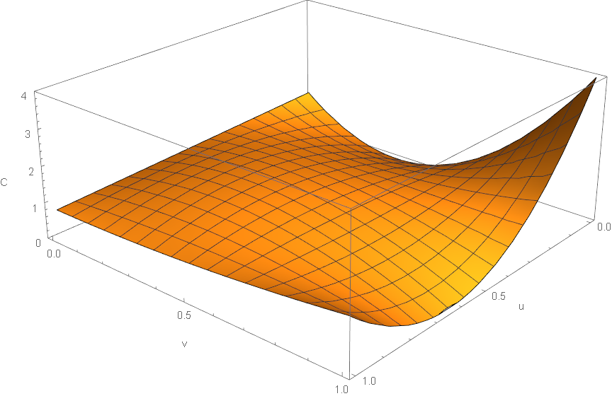
Fig 2: Plot of the density of Nelsen copula with ![]() .
.
For ![]() -many stocks, the test statistic
-many stocks, the test statistic ![]() can be calculated as follows for those that are interested:
can be calculated as follows for those that are interested:
(6) ![Rendered by QuickLaTeX.com \begin{align*} T & = n \mathbf{T}_{d,n}' \Sigma(\dot{c}_{\theta_0})^{-1} \mathbf{T}_{d,n} \stackrel{asymp}\sim \chi^2(q) \end{align*}, \quad \text{with} \\ \mathbf{T}_{d,n} = \mathbb{E}\left[ \frac{\partial}{\partial \theta} \log c_\theta (\mathbf{B}) \Bigg\vert_{\theta = \theta_0} \right], \quad \text{and} \\ \Sigma(\dot{c}_{\theta_0})_{i,j} = \int_{[0,1]^d} \left( \frac{\partial c_\theta(\mathbf{u})}{\partial \theta_i} \Bigg\vert_{\theta = \theta_0} \right) \times \left( \frac{\partial c_\theta(\mathbf{u})}{\partial \theta_j} \Bigg\vert_{\theta = \theta_0} \right) d \mathbf{u}](https://hudsonthames.org/wp-content/ql-cache/quicklatex.com-cf8c6aadcb4a208d11a210ec2505d8f7_l3.png)
It measures the ![]() deviation of
deviation of ![]() to
to ![]() . Note the above is a closed-form solution, so we are expecting a reasonably fast computation, especially when compared to the Genest test where simulation is needed.
. Note the above is a closed-form solution, so we are expecting a reasonably fast computation, especially when compared to the Genest test where simulation is needed.
Finally, the quadruple with the largest test statistic is considered the final quadruple for each target stock.
# Calculating final quadruples using the extremal approach for the first 10 target stocks.
extremal_Q = ps.extremal(10)
print(pd.Series(extremal_Q))
Output:
0           [A, TMO, PKI, DHR]
1         [AAL, UAL, DAL, ALK]
2         [AAP, GPC, PNR, DOV]
3    [AAPL, GOOG, GOOGL, MSFT]
4          [ABBV, A, TMO, DHR]
5         [ABC, MCK, CAH, WBA]
6       [ABMD, ISRG, ABT, BSX]
7        [ABT, BSX, SYK, ISRG]
8           [ACN, MA, V, VRSN]
9          [ADBE, MSFT, MA, V]
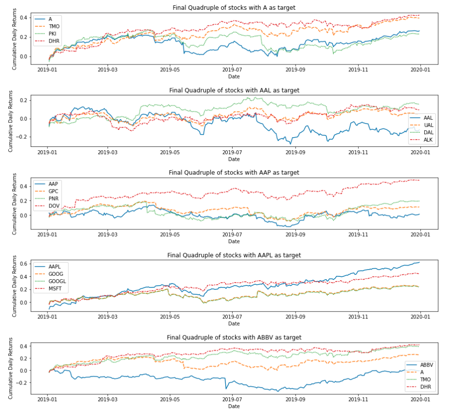
ps.plot_selected_pairs can be used to plot the cumulative daily returns of the stocks in the list of quadruples given as input.
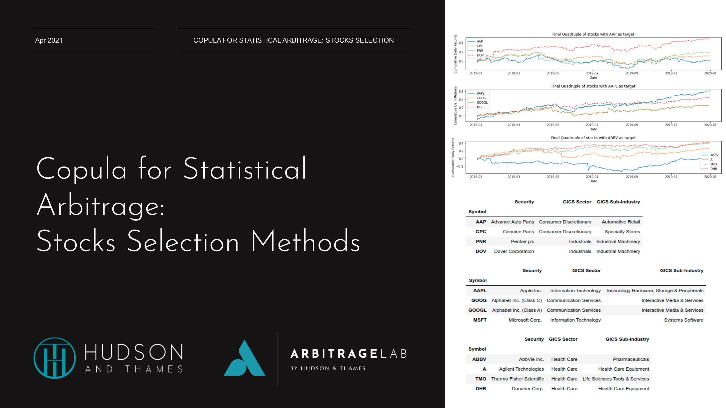
Fig 3: Cumulative Daily Return plots of five quadruples selected by the copula method.
ps.get_sector_data returns the name and sector data of stocks in the quadruple given as input.
Fig 4: Sub-Sector Data of five quadruples selected by the copula method.
Looking at the sector data, it becomes clear that the partners selected for the target stock are from similar industries and sub-sectors. Although we have not used any clustering techniques in the methodologies, we were still able to achieve good grouping. This result holds true for every multivariate method described above, which speaks for the value of these methods.
Comparing the results
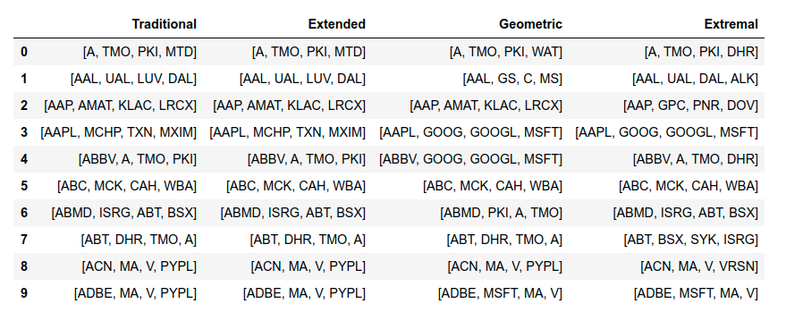
Fig 5: Comparison of Final Quadruples from multivariate methods.
The Traditional and Extended Methods seem to generate similar partners for each target stock. This is expected as both methods rely on a variation of Spearman’ s ![]() . The results from the Geometric approach show deviation from the Spearman’s approaches. Although this approach looks at the linear deviation in ranks like the previous two approaches, it does so using a distinctive technique that makes use of the relative distance of quadruples from the hyper-diagonal.
. The results from the Geometric approach show deviation from the Spearman’s approaches. Although this approach looks at the linear deviation in ranks like the previous two approaches, it does so using a distinctive technique that makes use of the relative distance of quadruples from the hyper-diagonal.
These three approaches were implemented in ArbitrageLab using vectorization techniques so the performance is pretty quick even on a comparatively basic machine.
Fig 6: Comparison of Spearman’s Approach to Geometric Approach for AAPL.
The results from the Extremal approach are quite varied in comparison to the other three approaches, which is expected. This copula-based approach primarily focuses on joint extreme events. Also, it is relatively heavy computationally compared to the other three, but still better than most simulation-based methods due to having a closed-form solution.
Fig 7: Comparison of other approaches to Extremal’s Approach for ABT.
What does it capture for copula trading methods?
Let us get back to our goal: when used for mean-reversion trading we aim to get groups of stocks that have a stable interdependent relationship such that one cannot deviate much from the others. If the stocks are independent then such a relationship will not occur. This test statistic can (in asymptotic) tell us whether the stocks are indeed independent or not (and thus dependent).
Moreover, due to the Nelsen copula’s structure, it is a test on whether the co-moves of extreme events (not necessarily in the same direction) happen more or less often than when they are independent. This is a very desirable property for copula-based methods in general.
A nuanced point that may be subject to criticism is that this test statistic ![]() can determine statistically significant independence relation, but a violation of independence does not necessarily lead to strong dependence, especially the desired type of dependence we want for a specific type of trading strategy. Nevertheless, it is still a great method for capturing co-moves in the tail. In the end, One needs to gain at least a qualitative understanding of this method before applying it.
can determine statistically significant independence relation, but a violation of independence does not necessarily lead to strong dependence, especially the desired type of dependence we want for a specific type of trading strategy. Nevertheless, it is still a great method for capturing co-moves in the tail. In the end, One needs to gain at least a qualitative understanding of this method before applying it.
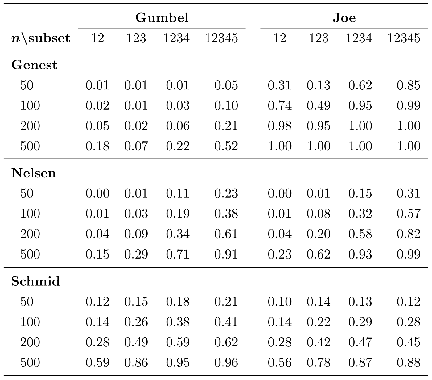
The power of the Nelsen copula test, the Genest test, and the Schmid test (n-dim Spearman’s ![]() ) used on simulated Gumbel and Joe copulas are listed below for reference:
) used on simulated Gumbel and Joe copulas are listed below for reference:
Table 1 from [Mangold 2016]. Simulated copulas have ![]() , a weak dependence relation.
, a weak dependence relation.
Comments
In the methods mentioned above, to reduce the computational burden, we only consider the top 50 most highly correlated stocks from the S&P 500 as potential partner stocks for a target stock. Creating curated methods for copula-based trading strategies is in general a difficult task. We went through why the difficulty comes from flexibility, and we listed a few common approaches that are readily available. Then we discussed in detail a copula-based method that specializes at capturing tail co-moves, potentially providing better tradable candidates for most copula-based strategies. In general, one has to understand what the copula strategy intrinsically is asking, then select one that best fits the purpose. We expect more developments in this area as copula-based trading methods get more popular.
References
- Luepsen, H., 2018. Comparison of nonparametric analysis of variance methods: A vote for van der Waerden. Communications in Statistics-Simulation and Computation, 47(9), pp.2547-2576.
- Mangold, B., 2015. A multivariate linear rank test of independence based on a multiparametric copula with cubic sections. FAU Discussion Papers in Economics (10).
- Nelsen, R.B., 2007. An introduction to copulas. Springer Science & Business Media.
- Rad, H., Low, R.K.Y. and Faff, R., 2016. The profitability of pairs trading strategies: distance, cointegration and copula methods. Quantitative Finance, 16(10), pp.1541-1558.
- Schmid, F. and Schmidt, R., 2007. Multivariate conditional versions of Spearman’s rho and related measures of tail dependence. Journal of Multivariate Analysis, 98(6), pp.1123-1140.
- Schmid, F. and Schmidt, R., 2007. Multivariate extensions of Spearman’s rho and related statistics. Statistics & probability letters, 77(4), pp.407-416.
- Stübinger, J., Mangold, B. and Krauss, C., 2018. Statistical arbitrage with vine copulas. Quantitative Finance, 18(11), pp.1831-1849.

