Mean-Reverting Spread Modeling: Caveats in Calibrating the OU Process

by Hansen Pei

Mean-Reverting Spread Modeling Cover Image

Join the Reading Group and Community: Stay up to date with the latest developments in Financial Machine Learning!

This is a series where we aim to cover in detail various aspects of the classic Ornstein-Uhlenbeck (OU) model and the Ornstein-Uhlenbeck Jump (OUJ) model, with applications focusing on mean-reverting spread modeling under the context of pairs trading or statistical arbitrage. Given the universality and popularity of those models, the techniques discussed can easily be applied to other areas where the OU or OUJ model seems fit.

Introduction

In this article, we aim to dive into the classic OU model, and illustrate the most common tasks encountered in applications:

1. How to generate an OU process.
2. Caveats in fitting an OU process.

The stochastic differential equation for an OU process is as follows:

$dX_t = \theta(\mu - X_t)dt + \sigma dW_t,$

where $\theta$ is the mean-reverting speed, $\mu$ is the long-term average and where the process reverts to, $W$ is a standard Wiener/Brownian process and $\sigma$ is the scaling for it (therefore the standard deviation for the Brownian part). Here $\theta, \mu, \sigma$ are positive constants, though in more generalized models they could vary with time.

The OU process is probably the simplest continuous-time mean-reverting model. Due to its simplicity, it is widely used across many fields in quantitative finance such as risk management, interest rate model, and pairs trading. It seems like a well-studied field that most problems are solved (like linear regression or linear algebra). However, lots of the common problems practitioners face are only recently treated with rigor, or not dealt with at all.

We start by presenting Doob’s exact method for generating an OU process. Then, we demonstrate that when one tries to fit an OU process, as we will see, the mean-reversion speed is in general notoriously difficult to estimate correctly.

Generating OU Process

Monte-Carlo methods are heavily used in analyzing stochastic processes and thus it is in general helpful to know how to simulate OU processes. The Monte-Carlo simulation also helps us understand the properties of the OU process itself, and they are heavily tied to the model’s parameter calibration as well, as we will see later.

Euler Scheme and Evaluating Stochastic Integral

Generally speaking, there are two ways for generating an OU process: Using an Euler advancement scheme (the Euler-Maruyama discretization) or using Doob’s exact simulation method. The former method is self-evident and quick to implement by directly looking at the OU process SDE. This is sure to introduce discretization errors (it is widely used anyway due to simplicity nevertheless).

An alternative approach is by looking at the analytical solution from the OU process:

$X_t = X_0 e^{-\theta t} + \mu(1 - e^{-\theta t}) + \sigma e^{-\theta t} \int_0^t e^{\theta s} dW_s.$

Only the last stochastic integral term is not deterministic. This integral when evaluated discretely, for example in the Ito’s sense (evaluate at the start of each integral), introduces error. One can divide the interval $(0, t)$ finely for less discretization error, but this increases computation time.

Also, generally one wishes to get a series of values $\{X_t\}$ where $t$ is on a grid: $0=t_0<t_1<...<t_n = T$ . The deterministic part can be pre-computed to save time, and pre-computation results in less discretization error, since the deterministic part of $X_t$ can be computed exactly. For the stochastic past, if the difference $\Delta^i t = t_i - t_{t-1}$ is small enough, one may simply approximate the stochastic integral (in the Ito’s sense) in one step by:

$\int_{t_{i-1}}^{t_i} e^{\theta s} dW_s \approx e^{\theta t_{i-1}} \sqrt{t_i - t_{i-1}} W.$

with $W \sim \mathcal{N}(0,1)$ .

Exact Simulation

This method is originally introduced and proved in [Doob (1942)]. For $0 < u < t$ we look at the analytical solution:

$X_t = e^{-\theta(t-u)} X_u + \mu \left( 1-e^{-\theta(t-u)} \right) + \sigma \int_u^t e^{-\theta(t-s)} dW_s.$

Reading from the above equation, we can treat $X_t$ as a random variable. Given $X_u$ , Doob proved the convenient result that $X_t$ is normally distributed with the mean being the deterministic part

$\mu_w(u,t) = e^{-\theta(t-u)} X_u + \mu(1-e^{-\theta(t-u)})$

and the variance coming from the random part

$\sigma_w^2(u,t) = \sigma^2 \int_u^t e^{-2\theta(t-s)} ds = \frac{\sigma^2}{2\theta}\left( 1 - e^{-2 \theta(t-u)}\right).$

Therefore, knowing $X_u$ , to simulate $X_t$ exactly, we have

$X_t = e^{-\theta(t-u)} X_u + \mu(1-e^{-\theta(t-u)}) + \sigma_w(u,t) W$

with $W \sim \mathcal{N}(0,1)$ . Notice this scheme can be computed as fast as the simple Euler-Maruyama discretization, just swap the Brownian increment at each step

$\text{from} \quad \sigma \sqrt{\Delta t} W \quad \text{to} \quad \sigma \sqrt{\frac{1 - e^{-2 \theta \Delta t}}{2 \theta}} W.$

And we can see that the discretization error comes from approximating $\frac{1 - e^{-2 \theta \Delta t}}{2 \theta}$ by $\Delta t$ , because it is only first-order accurate. The increment in simulation accuracy is huge. And practitioners should seriously consider the exact method.

Estimating Parameters

There are three constants to estimate: the mean-reverting speed $\theta$ , the long-term average $\mu$ , and the standard deviation $\sigma$ . In general, $\mu$ and $\sigma$ can be estimated relatively accurately with a reasonably large amount of observations (more than 250).

However estimating $\theta$ accurately is notoriously difficult, even with a large number of observations (more than 10000, that is more than one month of 1-min data for stocks). For pairs-trading applications, the mean-reverting speed is highly related to the profitability of strategies: We want $\theta$ to be large so that there are more mean-reverting behaviors. Moreover, a lot of analyses are based on the half-life of mean reversion, which for an OU process is just

$H = \frac{ln(2)}{\theta}.$

Methods for Parameter Estimation

AR(1) Approach

The most common approach is to treat the discrete data from an OU process as an AR(1) process and estimate the two parameters accordingly. The AR(1) process with constant time advancement $\Delta t$ is

$X_i = \alpha + \phi X_{i-1} + \sigma_\epsilon W_i.$

Therefore one can simply conduct a linear regression to find $\hat\alpha$ , $\hat\phi$ and $\hat\sigma_\epsilon$ . Rewrite the above equation into the following form to compare with the OU parameters:

$X_i - X_{i-1} = \alpha + (\phi-1) X_{i-1} + \sigma_\epsilon W_i.$

We have the estimated OU parameters as follows:

$\hat\theta = \frac{1-\hat\phi}{\Delta t}, \quad \hat\sigma = \sqrt{\frac{\sigma^2_{\epsilon}}{\Delta t}}, \quad \hat\mu = \frac{\hat\alpha}{1 - \hat\phi}.$

Here, $\sigma^2_\epsilon$ is the mean squared error of the residuals from the OLS. Since we are using OLS, we can directly look at the analytical solution for the coefficient $\hat\phi$ :

$\hat\phi = \frac{\sum_{i=1}^N (X_i-\hat\alpha) (X_{i-1}-\hat\alpha)}{\sum_{i=1}^N (X_{i-1}-\hat\alpha)^2}.$

And we can do slightly better by using the max likelihood estimator instead [Tang and Chen (2009)]:

$\hat\theta = - \frac{\ln(\hat \phi)}{\Delta t}.$

For the result, usually, there is not much difference compared to the direct AR(1) approach by choosing the max likelihood estimator, because the original data and its lag-1 are extremely similar, and $\hat \phi \approx 1$ . Therefore $\ln(\hat \phi) \approx \hat\phi - 1$ .

AR(1) Approach with Known Mean

When the long-term mean of the process is known, the AR(1) approach’s result can be enhanced:

$\hat\phi = \frac{\sum_{i=1}^N X_i X_{i-1}}{\sum_{i=1}^N X_{i-1}^2}, \quad \hat\theta = - \frac{\ln(\hat \phi)}{\Delta t}.$

The other 2 variables are the same as above. Readers familiar with simulations may already observe that this estimator comes from the exact simulation discussed above. When modeling a mean-reverting spread from a pair of prices, typically the long-term mean is 0. Therefore this assumption is not far-fetched.

The exact distribution of $\hat{\theta}$ is studied in [Bao et al. (2015)] under various realistic conditions: known or unknown $\mu$ , fixed or random initial value, etc. For realistic applications where samples are always finite, this estimator always has a positive bias. When applied to pairs trading, it means this method in general overestimates the mean-reverting frequency in any given period. We will discuss the bias in a later part of this article.

Direct Max-Likelihood

Still, assume $\mu=0$ . Stübinger et al. (2017) utilize the following method that directly uses the maximum likelihood of $(\theta, \sigma)$ conditioned on the (sequential) data. First, we directly look at the exact discretization of the OU process:

$X_t = e^{-\theta \Delta t} X_{t-1} + \sigma \sqrt{\frac{1 - e^{-2 \theta \Delta t}}{2 \theta}} W$

Again, this uses Doob’s result, and we have $X_t$ distributing normally with mean $e^{-\theta \Delta t} X_{t-1}$ and standard deviation $\sigma_w = \sigma \sqrt{\frac{1 - e^{-2 \theta \Delta t}}{2 \theta}}$ . That is, the conditional density given $X_{t-1}$ is a normal distribution:

$f(X_{t} | X_{t-1}; \theta, \sigma) = \frac{1}{\sigma_w \sqrt{2 \pi}} \exp\left[ -\frac{(X_{t} - X_{t-1}e^{-\theta \Delta t})^2}{2 \sigma_w ^2} \right].$

We now compute the sum of log-likelihood (in the sequential sense) given our sample data:

$\mathcal{L}(\theta, \sigma | X_1, \dots X_N) = -\frac{N \ln(2N)}{2} - N \ln(\sigma_w) - \frac{1}{2\sigma_w^2}\sum_{t=1}^N (X_t - X_{t-1}e^{-\theta \Delta t})^2.$

Then one can use a suitable optimization algorithm to maximize $\mathcal{L}$ , for example by gradient descent or L-BFGS-B. This approach is in general quite slower than the AR(1)-based methods discussed above, and under a pure OU process, it produces identical results to the AR(1) estimator with a known mean.

Moment Estimation Approach

This is adapted from a method proposed by Holý and Tomanová (2018): Take a look at the Doob’s exact discretization of the continuous OU process

$X_t = e^{-\theta(t)} X_0 + \mu \left( 1-e^{-\theta(t)} \right) + \sigma \int_0^t e^{-\theta(t-s)} dW_s.$

From Doob’s proof for the exact discretization, and also assume $X_0 \sim \mathcal{N}(\mu, \sigma^2 / 2\theta)$ , it turned out that $X_t$ is normally distributed with the following moments (all are unconditioned, because of our convenient choice of $X_0$ .):

(1) $\begin{align*} \mathbb{E}[X_t] &= \mu \\ \text{Var}[X_t] &= \frac{\sigma^2}{2\theta} \\ \text{Covar}[X_t, X_s] &= \frac{\sigma^2}{2\theta} e^{-\theta|t-s|}, \quad t \neq s. \end{align*}$

Assume we know the true mean $\mu = 0$ , then we can calculate the estimator:

$\hat \phi = \frac{\text{Covar}[X_i, X_{i-1}]}{\text{Var}[X_i]}, \quad \hat \theta = -\frac{\ln(\hat \phi)}{\Delta t}$

where we need to use unbiased estimators for the variance and covariance. After some algebra work we arrive at (note that we have $N+1$ total instances):

$\hat\phi = \frac{\sum_{i=1}^N X_i X_{i-1}}{\sum_{i=1}^N X_{i-1}^2} \frac{N}{N-1}, \quad \hat\theta = - \frac{\ln(\hat \phi)}{\Delta t}.$

You will be surprised at how much difference this adjustment makes for not-so-large $N$ . Since the max-likelihood estimator always has a positive bias, this adjustment makes the bias less pronounced by effectively subtracting a positive term $\ln(\frac{N}{N-1}) / \Delta t$ from it. Also $\Delta t$ and $\ln(\frac{N}{N-1})$ are in general at the same order of magnitude, making this term not negligible.

At this stage, the reader might ask whether we are splitting hairs, or are just playing with the regression coefficients from the OLS. Indeed, if we have infinite samples, all of the above four methods (practically only three are different) coincide as one should expect, and they do not have any bias. However, for finite samples, they result in very different bias profiles, especially when $\theta$ is small.

Can We Do Better?

Well, if we know the data do come from a pure OU process (no added noise, no jumps, etc.), it is quite challenging to form an estimator for $\theta$ that can outperform those estimators. They all directly look at the distributions at each time step of the OU process by taking full advantage of its normal distribution and extracts the coefficients from there.

For improvements, one needs to look beyond the AR(1) and the moment method. To the best of our knowledge, the indirect inference estimation is unbiased for finite samples. However, this method is simulation-based and is relatively slow. Interested readers can refer to [Phillips and Yu, (2008)] for details.

Asymptotic Distributions of Theta Estimator

The estimator $\hat\theta$ from the AR(1) method with known mean is the most thoroughly studied one in mathematical statistics. It coincides with the direct max-likelihood estimator. Since $\hat\theta$ can be quite inaccurate (in the sense of bias and variance), one may want to take a step back and look at the full distribution of $\hat\theta$ to quantify the uncertainty. [Bao et al. (2015)] found the exact distributions of this estimator. However, the details are rather technical and we will skip those for this introductory post. One without access to the analytical solution can directly use Monte-Carlo to generate the distribution with reasonable speed. Let’s look at some of the asymptotic distributions listed in [Zhou and Yu (2015)] [Bao et al. (2015)] for different scenarios. Assume the true $\theta>0$ , and we have the discrete data of an OU process in time $[0, T]$ with constant increment $\Delta t$ . The last case for fixed $T$ has relatively complicated expressions, and interested readers can refer to the original works.

⠀
$T \rightarrow \infty$ , $\Delta t$ fixed
$T \rightarrow \infty$ , $\Delta t \rightarrow 0$
$T$ fixed, $\Delta t \rightarrow 0$

$\mu=0$
$\sqrt{T}(\hat\theta - \theta) \xrightarrow{d} \mathcal{N}(0, \frac{e^{2\theta \Delta t}-1}{\Delta t})$
$\sqrt{T}(\hat\theta - \theta) \xrightarrow{d} \mathcal{N}(0, 2 \theta)$
See the original works

$\mu$ Unknown
$\sqrt{T}(\hat\theta - \theta) \xrightarrow{d} \mathcal{N}(0, \frac{e^{2\theta \Delta t}-1}{\Delta t})$
$\sqrt{T}(\hat\theta - \theta) \xrightarrow{d} \mathcal{N}(0, 2 \theta)$
See the original works

Thus, whether $\mu$ is $0$ or not, asymptotically for infinite $T$ , we do get unbiased estimations, but even with the best case where $T \rightarrow \infty$ , $\Delta t \rightarrow 0$ , the standard deviation of $\hat \theta - \theta$ only decreases by $\sqrt{T}$ . The convergence is quite slow. However, when $T$ is fixed, even if we let $\Delta t \rightarrow 0$ , we still have a bias in the estimator. This makes sense, because, say we have only 2 days of data from a spread, and the spread has its half-life of mean reversion being a month, the information we get within these 2 days is very limited, no matter how much high-frequency data we have access to for this pair of instruments.

Estimating the Bias of Theta Estimate

Constructing the exact analytical solution from [Bao et al. (2015)] can be a quite involving exercise even given the manual, as it requires an understanding of joint characteristic functions and details in the numerical integration of complex functions. Yu (2009) investigated a quick way to approximate the bias with second order-accuracy:

$\mathbb{E}[\hat \theta] - \theta = \frac{1}{2T}(3+e^{2\theta \Delta t}) - \frac{2(1-e^{-2 \theta T})}{T N (1-e^{-2 \theta \Delta t})}$

where $N = T/\Delta t$ . Unfortunately to the best of our effort, we are unable to fully replicate this result at low values of $\theta$ , since the result is extremely sensitive to the underlying assumptions.

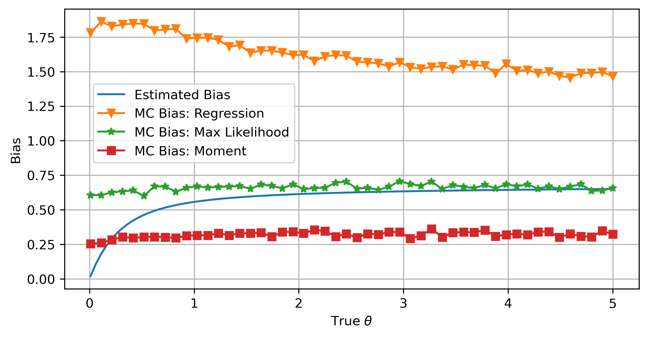
Below we compare the bias generated from the three different estimation methods of $\theta$ . Each plotted point is an average of 10000 Monte-Carlo results. We take $\sigma=0.1$ , $\Delta t = 1/252$ , and $N=756$ to emulate having access to 3 years of daily data. As we can see, the more information we have, the less the bias: In the regression method, when we do not know the mean, it has the largest bias. When we know the mean is $0$ , the bias drops significantly. When we calculate the moments exactly, it has the lowest amount of bias.

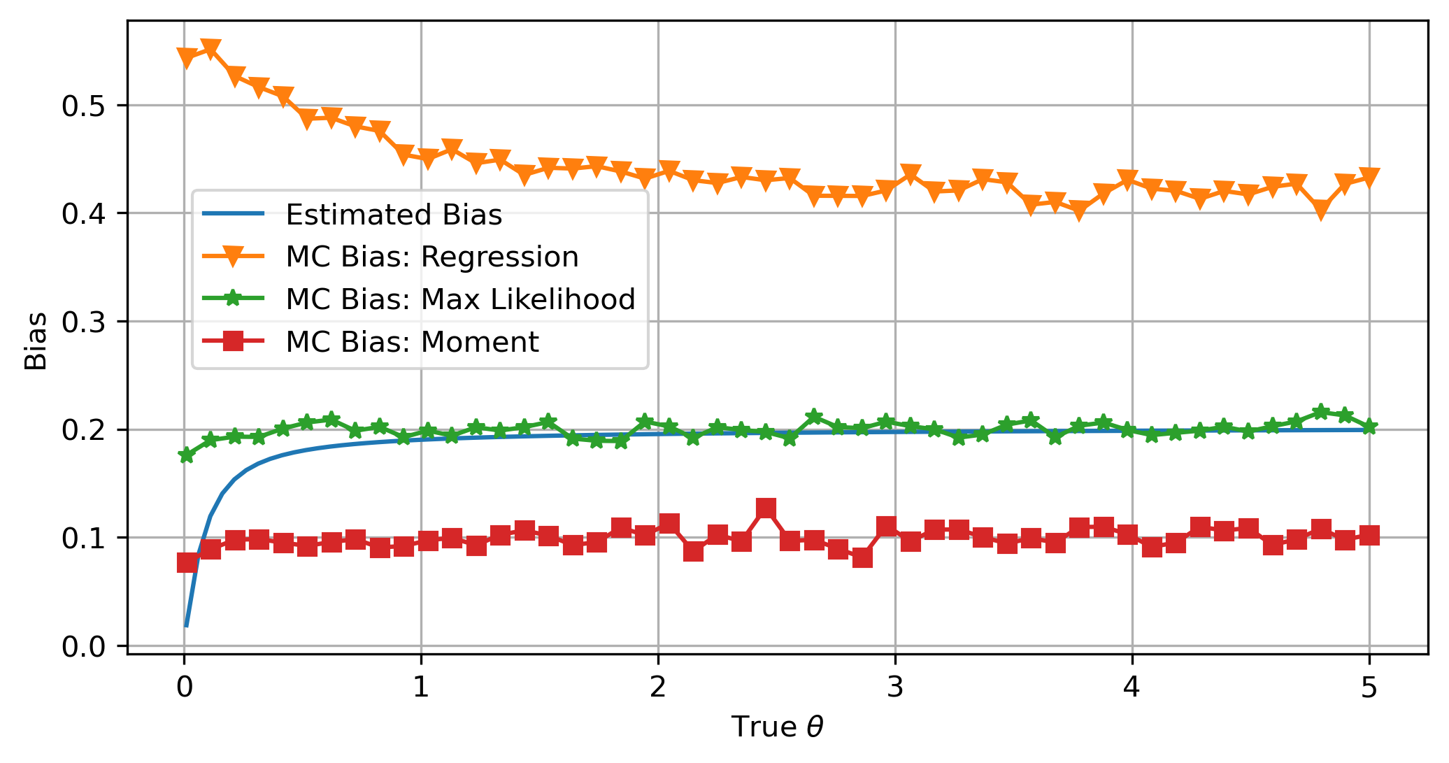
Now we assume $\sigma=0.1$ , $\Delta t = 1/391$ , and $N=3910$ to emulate having access to 10 days of 1-min data. We see that with an effectively larger time span, the overall bias decreases.

Noises and Jumps

Financial data generally have lots of noise, and it may contain jumps. Those two can seriously influence our model calibration. Here we talk briefly go over the major effects of our calibration from those two phenomena, but the details are left for another dedicated post to discuss.

The OU process with added noise still satisfies the original OU model SDE, however, our observations are assumed to be contaminated by Gaussian noise $E_i$ :

$X_i \leftarrow X_i + E_i, \quad E_i \sim \mathcal{N}(0, \omega^2).$

In this case, the estimator $\hat\theta$ and $\hat \sigma$ can have an infinite bias as $n \rightarrow \infty$ . In the work of [Holý and Tomanová, (2018)], they discussed several methods that can handle the added noise.

When jumps are present, generally the process is modeled as an OU-Jump process:

$dX_t = \theta(\mu - X_t) dt + \sigma dW_t + \ln (J_t) d N_t,$

where $\ln(J_t)$ the jump size is normally distributed, and $N_t$ is a Poisson arrival process. The jumps lead to significant fat tails in the distribution of $X_t$ and as a result, the OU process data is no longer normally distributed. If we blindly apply the OU estimation methods, both $\hat\theta$ and $\hat\sigma$ will severely overestimate their true value on average. Thus the jumps need to be filtered before applying the OU estimation. In the works of [Mai, (2012)], [Cartea and Figueroa, (2007)], [Cázares and Ivanovs, (2020)], several techniques for filtering the jumps are discussed in detail, and this seemingly straight-forward jump-filtering procedure is far from trivial.

Monte-Carlo Results

Experiment 1

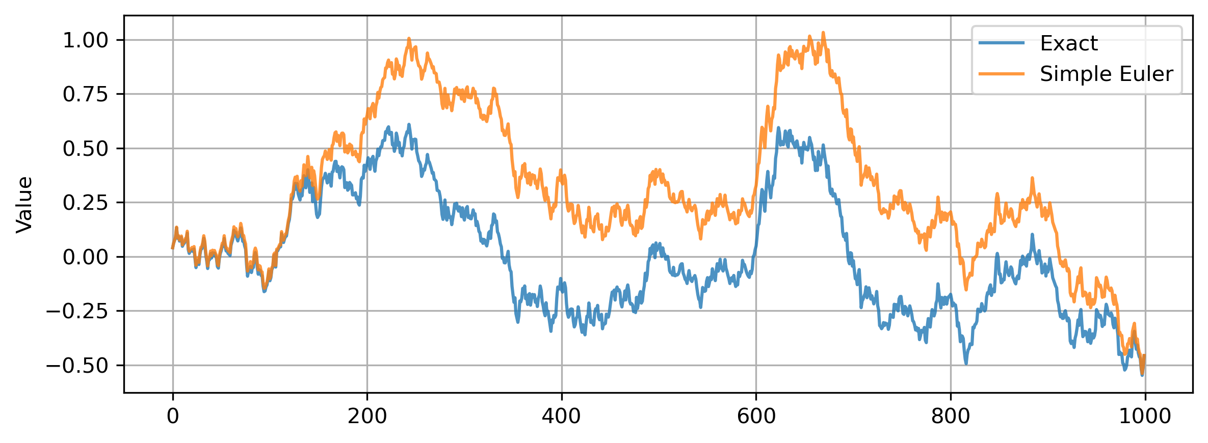
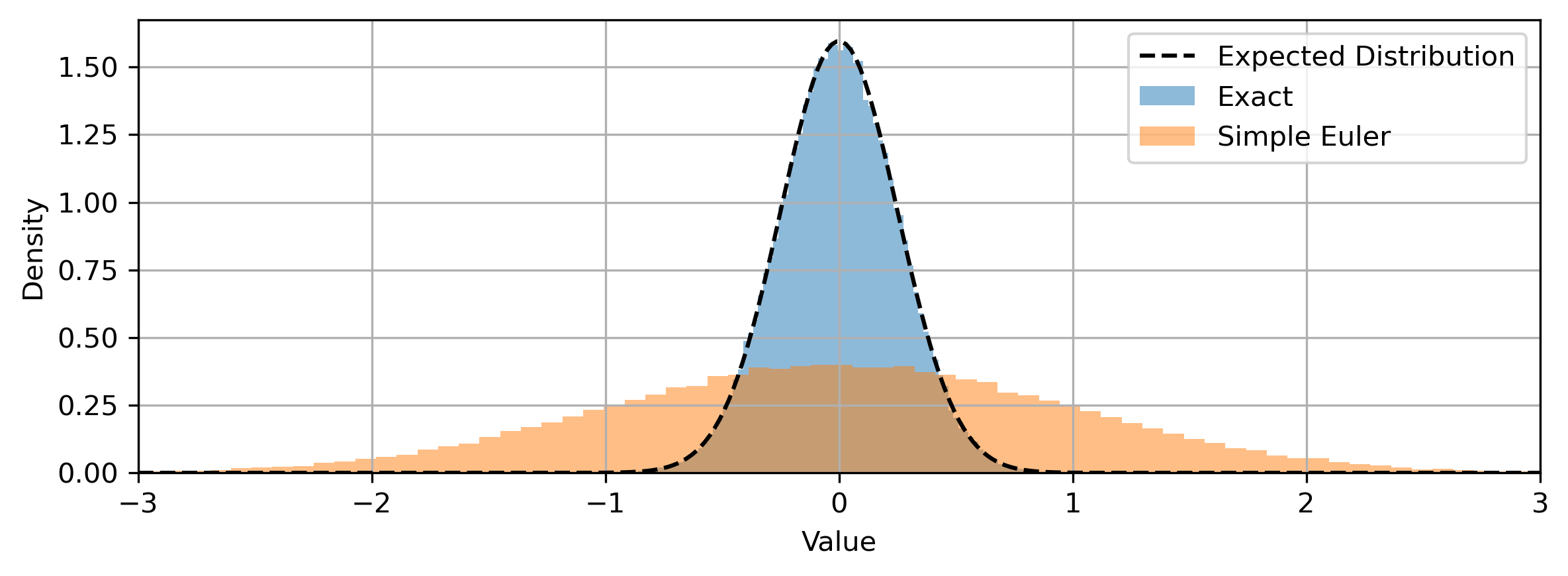
We compare the Euler-Maruyama discretization scheme with Doob’s exact simulation scheme. The two methods utilize the same Gaussian noise for direct comparison. The parameters used are: $\theta=2$ , $\mu=0$ , $\sigma=0.5$ , $\Delta t=1/252$ , $N=1000$ . We can see that there is a noticeable difference. The order 1 discretization error accumulates because each step depends on its previous step.

Now we look at their distributions at the end of the simulation:

Experiment 2

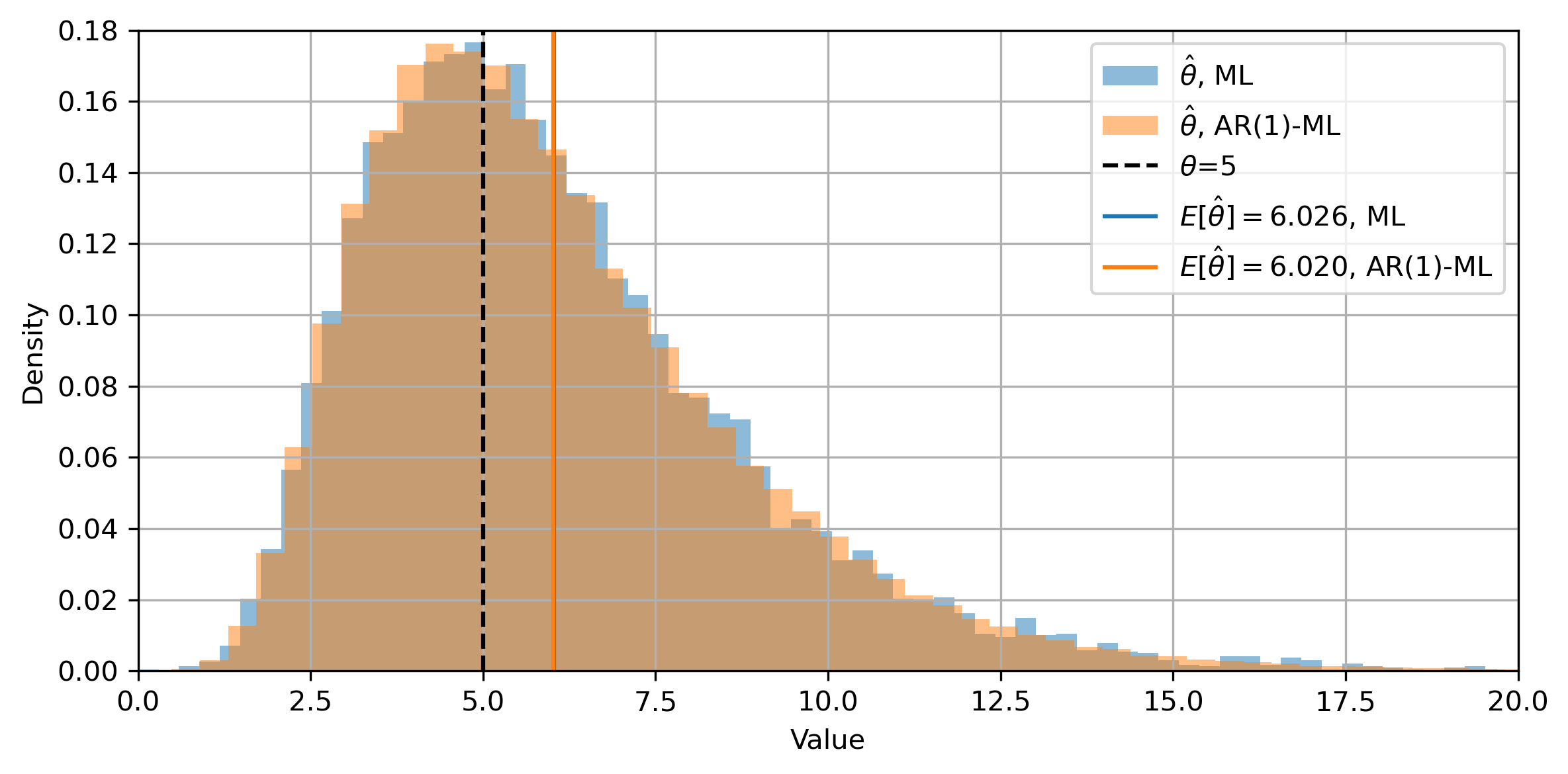
For the rest of the experiments, We simulate the OU process exactly and use them to see the distribution of the estimator from AR(1) with a known mean. First, we use the direct ML estimation and compare it with the AR(1) method. The density plot is rather coarse because we only use 10000 Monte-Carlo paths for estimation for this method being relatively slow. The two estimations produce almost identical results.

Experiment 3

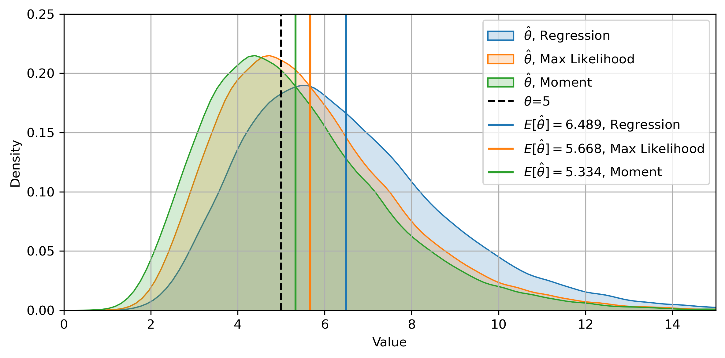
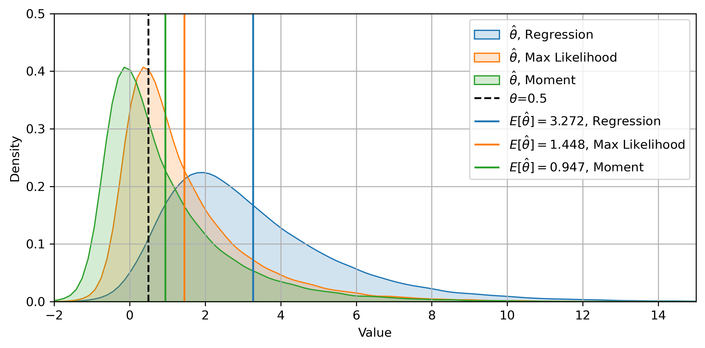
We directly look at the distributions from the three different methods for large $\theta$ and small $\theta$ . We change the KDE plot style for a clearer view. First, we have $\theta=5$ , $\Delta t=1/252$ , $N = 756$ . This is one of the nicer cases and we can see the three methods mostly agree with each other.

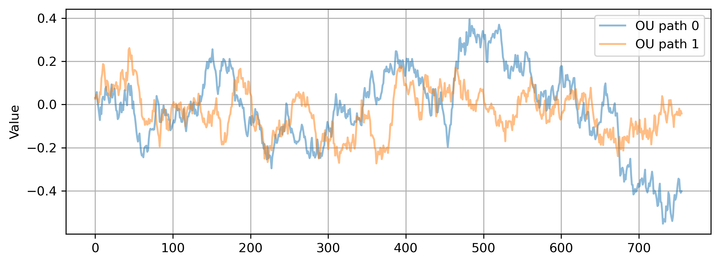
Here are some of the simulated OU paths. The half-life of mean reversion is relatively small.

Experiment 4

Then, we have $\theta=0.5$ , $\Delta t=1/252$ , $N = 504$ . We can see that the relative bias grows larger, and we even have a great portion of our estimation such that $\hat\theta < 0$ . Also, the discrepancies among the three methods enlarge by quite a lot. This further demonstrates the point that, when $\theta$ is small, we should take the estimation with a grain of salt.

Key Takeaways

Here are some of the major takeaways:

1. We can generate an OU process exactly at pretty much no extra cost.
2. The estimator for $\theta$ is biased and often has a large variance for AR(1)-based methods, and in principle, this is very difficult to improve. Since $\theta$$ is often overestimated, under a pairs trading scenario, the model is often too optimistic, because faster mean-reversion indicates more profit.
3. The direct max-likelihood method produces identical results to the AR(1) method with a known mean using a max-likelihood estimator. But it is quite slower.
4. Two situations where we should not trust the estimations very much: 1. If the mean-reverting speed is small, or equivalently the half-life of mean-reversion is large (e.g. less than 20 crosses of mean in the timespan); 2. If the sample size is not large enough (e.g., less than 1 year of end-of-day data). Realistically in some scenarios, it is quite difficult to achieve either.
5. Estimations for $\sigma$ and $\mu$ are in general much more reliable than $\theta$ .
6. Noises and jumps can further complicate the situation and need to be dealt with carefully.

References

- Bao, Y., Ullah, A. and Wang, Y., 2017. Distribution of the mean reversion estimator in the Ornstein–Uhlenbeck process. Econometric Reviews, 36(6-9), pp.1039-1056.
- Cartea, A. and Figueroa, M.G., 2005. Pricing in electricity markets: a mean reverting jump diffusion model with seasonality. Applied Mathematical Finance, 12(4), pp.313-335.
- Casella, B. and Roberts, G.O., 2011. Exact simulation of jump-diffusion processes with Monte Carlo applications. Methodology and Computing in Applied Probability, 13(3), pp.449-473.
- Doob, J.L., 1942. The Brownian movement and stochastic equations. Annals of Mathematics, pp.351-369.
- Grimmett, G. and Stirzaker, D., 2020. Probability and random processes. Oxford university press.
- Gloter, A., Loukianova, D. and Mai, H., 2018. Jump filtering and efficient drift estimation for Lévy-driven SDEs. The Annals of Statistics, 46(4), pp.1445-1480.
- Glasserman, P., 2013. Monte Carlo methods in financial engineering (Vol. 53). Springer Science & Business Media.
- Holý, V. and Tomanová, P., 2018. Estimation of Ornstein-Uhlenbeck Process Using Ultra-High-Frequency Data with Application to Intraday Pairs Trading Strategy. arXiv preprint arXiv:1811.09312.
- Mai, H., 2012. Drift estimation for jump diffusions.
- Meyer-Brandis, T. and Tankov, P., 2008. Multi-factor jump-diffusion models of electricity prices. International Journal of Theoretical and Applied Finance, 11(05), pp.503-528.
- Phillips, P.C. and Yu, J., 2009. Maximum likelihood and Gaussian estimation of continuous time models in finance. In Handbook of financial time series (pp. 497-530). Springer, Berlin, Heidelberg.
- Stübinger, J. and Endres, S., 2018. Pairs trading with a mean-reverting jump–diffusion model on high-frequency data. Quantitative Finance, 18(10), pp.1735-1751.
- Yu, J., 2012. Bias in the estimation of the mean reversion parameter in continuous time models. Journal of Econometrics, 169(1), pp.114-122.
- Zhou, Q. and Yu, J., 2010. Asymptotic distributions of the least squares estimator for diffusion processes.