Discrimination of Correlated Random Walk Time Series using GNPR
By David Munoz Constantine
Join the Reading Group and Community: Stay up to date with the latest developments in Financial Machine Learning!
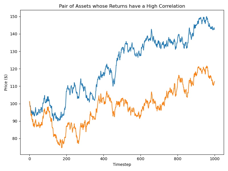
Discriminating random variables on time-series on both their distribution and dependence information is motivated by the study of financial assets returns. For example, given two assets where their returns are perfectly correlated, are these returns always similar from a risk perspective? According to Kelly and Jiang (2014), the answer is no, because we did not take into account the distribution differences and distribution information. Therefore, there is a need for a distance metric that can distinguish underlying distributions of time-series even if they are perfectly correlated.
Figure 1. Two asset time series whose returns have a Pearson’s correlation value > 0.8. They are not similar from a risk perspective.
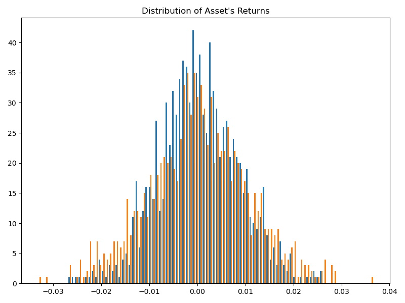
Figure 2. Two asset returns distributions whose returns have a Pearson’s correlation value > 0.8. They are not similar from a risk perspective.
Marti, Very and Donnat (2016) proposed the generic non-parametric representation (GNPR) and the generic parametric representation (GPR) distance metrics to accomplish this goal.
Normally distributed random variables can be separated by both the GNPR and GPR methods. To separate i.i.d. random variables with distributions other than normal, we can use the GNPR method. GNPR has good performance on discriminating time-series that have any embedded distribution. The relationship between two random variables can be roughly classified into two families (Marti, Very and Donnat, 2016):
- Distributional distances: It measures the similarity or dissimilarity between probability distributions.
- Dependence distances: It measures the joint behavior of random variables.
For example, if we have two time-series, where one exhibits a normal distribution, and the other exhibits a heavy-tailed distribution, they can be perfectly correlated with each other. Nevertheless, as stated in our earlier example, they are not similar from a risk perspective. Standard measures of similarity between random variables, such as Pearson’s correlation, Spearman’s rho correlation, cosine distance, and Euclidean distance, cannot fully distinguish multiple distributions in multiple time series.
A good separation of random variables is useful for basic clustering algorithms such as k-means, k-means++, ward hierarchical clustering, Gaussian mixture models, etc. When these algorithms are not given a suitable distance metric to separate clusters, their performance suffers considerably. GNRP is a solution to this problem by enhancing cluster separation.
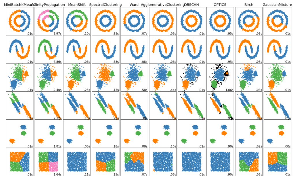
Figure 3. Various clustering methods. Naive implementations use the euclidean distance between points to separate them. What if the cluster’s relation is non-linear? (Courtesy of scikit learn)
Synthetic Clustered-Time-Series Generation
To verify the GNPR method’s performance, Marti, Very, and Donnat (2016) proposed an approach to generate correlated and clustered time-series. This approach can generate random variables that have different levels of distributional and dependence distances. Each time-series dataset can contain any number of time-series ( ![]() ). Each of these time series has the same number of time steps (
). Each of these time series has the same number of time steps ( ![]() ). To embed correlation distributions into these time series, we divide each time series into
). To embed correlation distributions into these time series, we divide each time series into ![]() correlation clusters. To embed dependence distributions into the time-series, we divide each correlation cluster into
correlation clusters. To embed dependence distributions into the time-series, we divide each correlation cluster into ![]() distribution clusters.
distribution clusters.
The authors provide multiple sample parameters and distributions in their paper to get started. In Table 1, ![]() represents the normal distribution,
represents the normal distribution, ![]() represents
represents ![]() , and
, and ![]() represents
represents ![]() .
.
Table 1. Sample parameters.
In this table, ![]() represents random distributions each of length
represents random distributions each of length ![]() , and
, and ![]() are independent random distributions of length
are independent random distributions of length ![]() .
.
The authors show that even though the mean and the variance of the ![]() and
and ![]() distributions are the same and their variables are highly correlated, GNPR can separate them into different clusters successfully.
distributions are the same and their variables are highly correlated, GNPR can separate them into different clusters successfully.
In our implementation, the available distributions from which ![]() and
and ![]() can sample from are:
can sample from are:
- Normal distribution (np.random.normal)
- Laplace distribution (np.random.laplace)
- Student’s t-distribution (np.random.standard_t)
We will demonstrate how these parameters can generate a dataset of time series, and how GNPR compares against other methods.
The three measures we will compare GNPR against are the distance correlation, Spearman’s rho, and GPR methods. Distance correlation captures both linear and non-linear dependencies, in contrast to Pearson’s correlation that only captures linear dependencies. Spearman’s rho is a copula-based dependence measure and captures linear and non-linear dependencies as well.
import matplotlib.pyplot as plt
from mlfinlab.data_generation.correlated_random_walks import generate_cluster_time_series
from mlfinlab.data_generation.data_verification import plot_time_series_dependencies
import numpy as np
np.random.seed(2814)
# Initialize the example parameters for each example time series.
n_series = 200
t_samples = 5000
k_clusters = [1, 10, 5]
d_clusters = [4, 1, 2]
rho_corrs = [0, 0.3, 0.3]
dists_clusters = [["normal",    "normal",    "laplace",   "student-t",
                  "normal_2"],
                  ["student-t", "student-t", "student-t", "student-t",
                   "student-t"],
                  ["normal",    "normal",    "student-t", "normal",
                   "student-t"]]

def plot_time_series(dataset, title, theta=0.5):
    """
    Helper function to plot a dataset timeseries and different distance
    metrics.
    """
    dataset.plot(legend=None,
                   title="Time Series for {} Example".format(title),
                   figsize=(9,5))

    plot_time_series_dependencies(dataset,
          dependence_method='distance_correlation')
    plot_time_series_dependencies(dataset,
          dependence_method='spearmans_rho')
    plot_time_series_dependencies(dataset,
          dependence_method='gpr_distance', theta=theta)
    plot_time_series_dependencies(dataset,
          dependence_method='gnpr_distance', theta=theta)
Distribution Clustering
The Distribution example generates a time series with global normal distribution, no correlation clustering, and four distribution clusters. The four distribution clusters include the Laplace distribution, Student-t distribution, normal distribution with a standard deviation of 1, and a normal distribution with a standard deviation of 2.
# Plot the time series and codependence matrix for the distribution example.
dataset = generate_cluster_time_series(n_series=n_series,
                      t_samples=t_samples, k_corr_clusters=k_clusters[0],
                      d_dist_clusters=d_clusters[0], rho_corr=rho_corrs[0],
                      dists_clusters=dists_clusters[0])

plot_time_series(dataset, title="Distribution", theta=0)
plt.show()
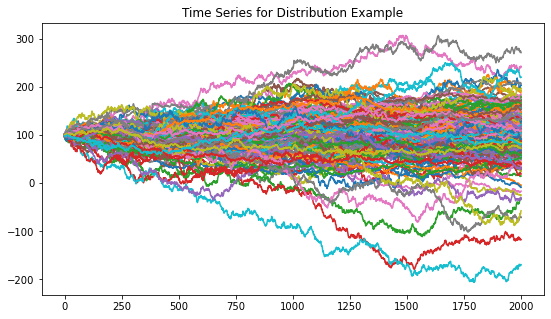
Figure 4. Resulting random walk time series dataset for the distribution example.
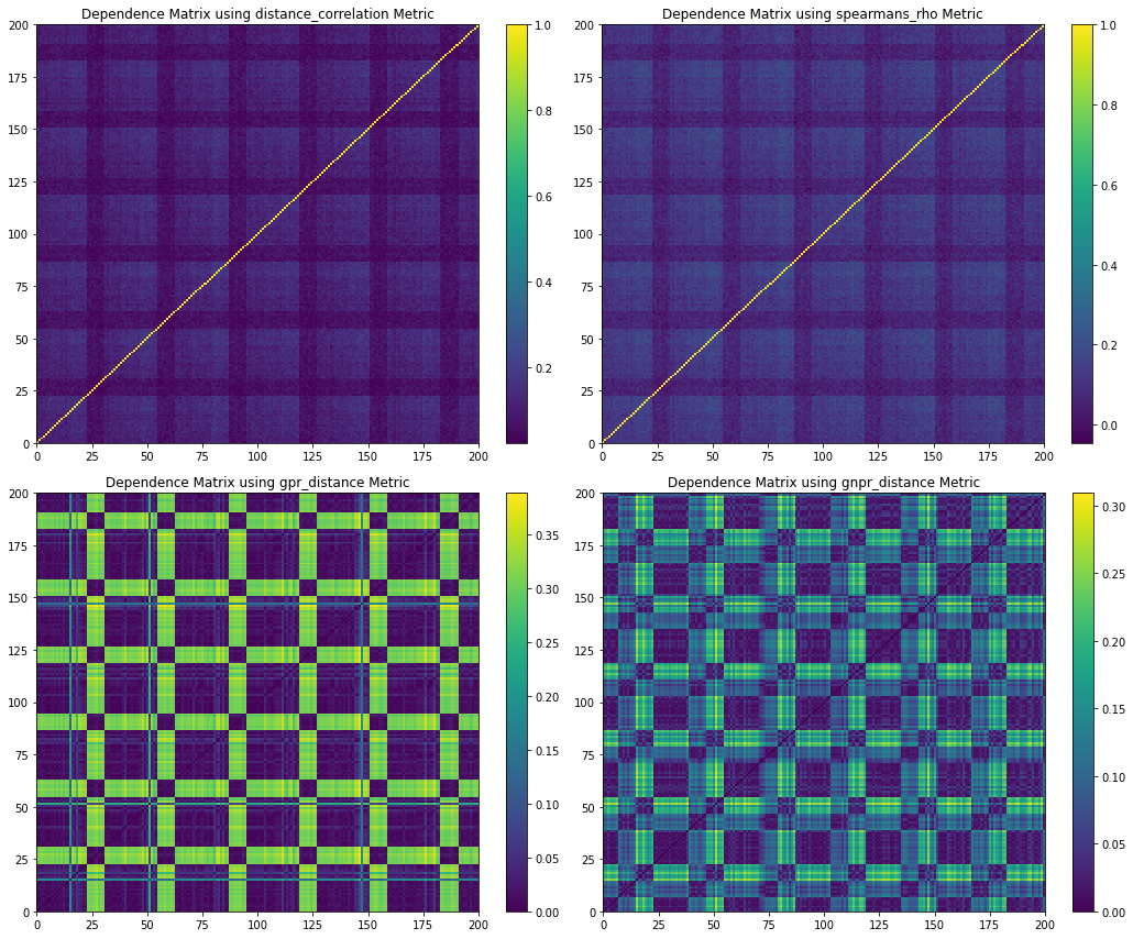
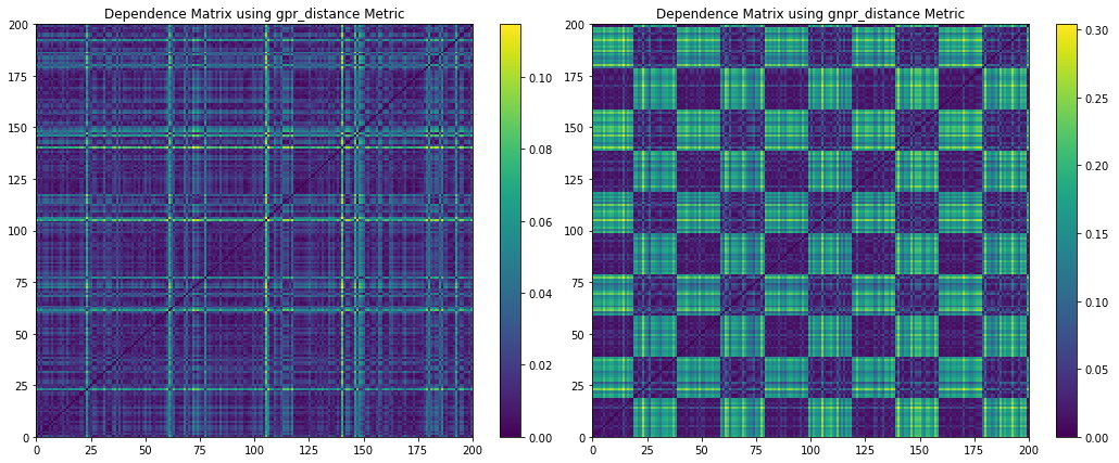
Figure 5. Codependence matrices generated using various distance methods with ![]() . Note how the GNPR method (lower right) can separate all the clusters.
. Note how the GNPR method (lower right) can separate all the clusters.
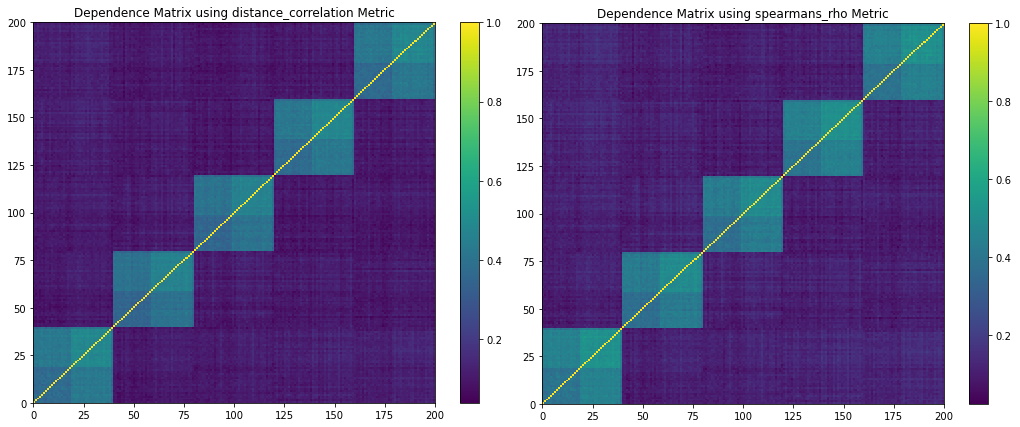
Figure 4 shows the random walk time series that is generated from the distribution example parameters. Figure 5 shows the codependence matrices generated from the time series dataset. The distance correlation and Spearman’s rho metrics are barely able to separate all 4 distributions clusters. The GPR method separates only 2 distributions clusters, and the rest of the clusters are barely visible. The GNRP dependence matrix shows the separation of the 4 distribution clusters. Since the distribution clusters contain two normal distributions with slightly different standard deviations, it is more difficult for GNPR to separate them perfectly.
Dependence Clustering
The Dependence example generates a time series with a global normal distribution, 10 correlation clusters with an underlying Student’s t distribution, and no distribution clusters.
# Plot the time series and codependence matrix for the dependence example.
dataset = generate_cluster_time_series(n_series=n_series,
                   t_samples=t_samples, k_corr_clusters=k_clusters[1],
                   d_dist_clusters=d_clusters[1], rho_corr=rho_corrs[1],
                   dists_clusters=dists_clusters[1])

plot_time_series(dataset, title="Dependence", theta=1)
plt.show()
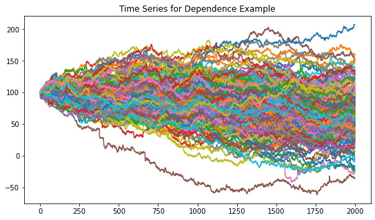
Figure 6. Resulting random walk time series dataset for the dependence example.
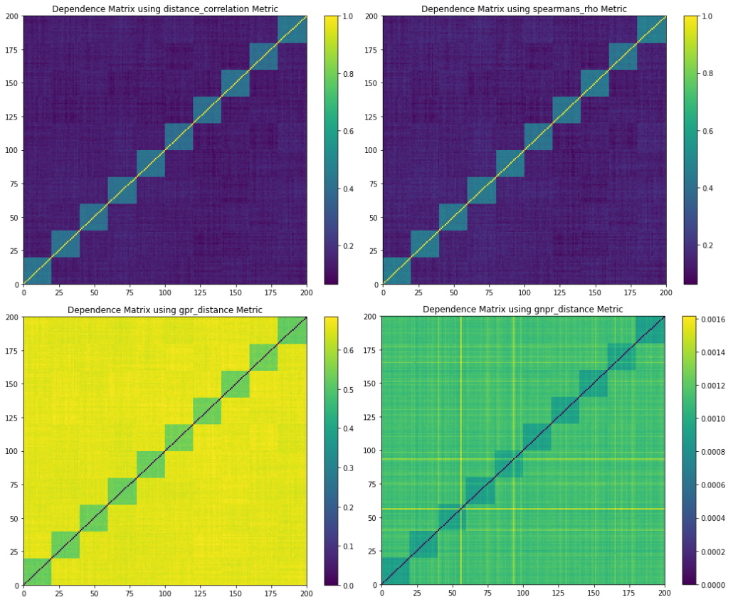
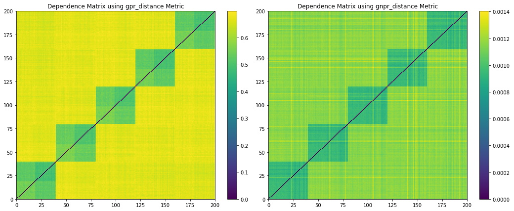
Figure 7. Codependence matrices generated using various distance methods with ![]() . Due to the correlation clusters having normal distribution, all methods are able to separate the correlation clusters.
. Due to the correlation clusters having normal distribution, all methods are able to separate the correlation clusters.
Figure 6 shows the random walk time series that are generated from the dependence example parameters. Figure 7 shows the codependence matrices generated from the time series dataset. All methods are able to separate the 10 correlation clusters.
Mix Clustering
This distribution example can be seen in the original work of the authors. So far, we have used a theta ( ![]() ) parameter for the GNPR method to be
) parameter for the GNPR method to be ![]() . This value represents which information to extract from the time series. Depending on its value, it extracts the following information:
. This value represents which information to extract from the time series. Depending on its value, it extracts the following information:
– distribution information ( ![]() )
)
– dependence information ( ![]() )
)
– a mix of both distribution and dependence information ( ![]() ).
).
The authors propose that ![]() “ideally should reflect a balance o dependence and distribution information in the data”. This implies that the
“ideally should reflect a balance o dependence and distribution information in the data”. This implies that the ![]() value chosen depends on the data being analyzed.
value chosen depends on the data being analyzed.
Below we show how the Mix time series, which has a global normal distribution, 5 correlation clusters, and 2 distribution clusters, are clustered depending on its ![]() value.
value.
# Plot the time series and codependence matrix for the mix example.
dataset = generate_cluster_time_series(n_series=n_series,
                   t_samples=t_samples, k_corr_clusters=k_clusters[2],
                   d_dist_clusters=d_clusters[2], rho_corr=rho_corrs[2],
                   dists_clusters=dists_clusters[2])

plot_time_series(dataset, title="Mix")
plt.show()
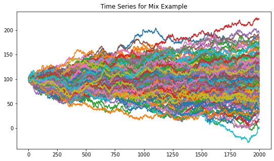
Figure 8. Resulting random walk time series dataset for the mix example.
Figure 9. Codependence matrices generated using the distance and Spearman’s rho distance methods. They are not able to fully separate all dependencies.
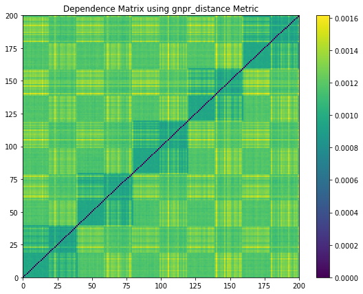
Figure 8 shows the random walk time series that are generated from the mix example parameters. Figure 9 shows the codependence matrices generated by the distance and Spearman’s rho distance metrics. Notice how these methods can only separate the 5 correlation clusters, missing the 2 distribution clusters and the global normal distribution.
Since only the GPR and GNPR methods accept the ![]() parameter, we will compare them with different theta values.
parameter, we will compare them with different theta values.
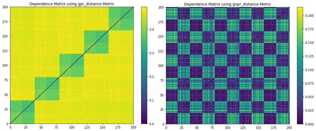
Figure 10. Codependence matrices generated using the GPR and GNPR methods with ![]() .
.
From Figure 10, we can observe when ![]() , the GPR codependence matrix has indistinguishable clusters. GNPR, on the other hand, can separate 10 clusters created from the 5 correlation and 2 distribution clusters. Note that without prior information on the embedded distributions, one cannot discern that there should be only 2 distribution clusters. No clear correlation clusters can be discerned.
, the GPR codependence matrix has indistinguishable clusters. GNPR, on the other hand, can separate 10 clusters created from the 5 correlation and 2 distribution clusters. Note that without prior information on the embedded distributions, one cannot discern that there should be only 2 distribution clusters. No clear correlation clusters can be discerned.
Figure 11. Codependence matrices generated using the GPR and GNPR methods with ![]() .
.
From Figure 11, we can observe when ![]() , both the GPR and GNPT codependence matrices separate 5 correlation clusters but fails to separate the distribution clusters. Emphasizing the need to pick the correct
, both the GPR and GNPT codependence matrices separate 5 correlation clusters but fails to separate the distribution clusters. Emphasizing the need to pick the correct ![]() value for each application.
value for each application.
Figure 12. Codependence matrices generated using the GPR and GNPR methods with ![]() .
.
From Figure 12, we can observe when the GPR codependence matrix has the same performance when ![]() , and the GNPR has the same performance when
, and the GNPR has the same performance when ![]() . This means GNPR separates 10 clusters, but there is no clear representation of all the embedded distributions. This means that for this dataset, we need a more accurate
. This means GNPR separates 10 clusters, but there is no clear representation of all the embedded distributions. This means that for this dataset, we need a more accurate ![]() value to observe clear discrimination of all distributions. Therefore, at which
value to observe clear discrimination of all distributions. Therefore, at which ![]() value the correlation and dependence distributions start to separate? After a few iterations, we found that when
value the correlation and dependence distributions start to separate? After a few iterations, we found that when ![]() we started to observe the distribution clusters being separated from the correlation clusters.
we started to observe the distribution clusters being separated from the correlation clusters.
Figure 13. Codependence matrix using the GNPR method with ![]() . The 5 correlation clusters in the diagonal are being separated from the 2 distribution clusters.
. The 5 correlation clusters in the diagonal are being separated from the 2 distribution clusters.
From Figure 13, we can observe when ![]() the GNPR method clearly separates each of the 5 correlation clusters along the main diagonal, and it starts to separate each of the correlation clusters into 2 distribution clusters. Without prior information on the embedded distributions, one can be more confident in their observation of the number of clusters.
the GNPR method clearly separates each of the 5 correlation clusters along the main diagonal, and it starts to separate each of the correlation clusters into 2 distribution clusters. Without prior information on the embedded distributions, one can be more confident in their observation of the number of clusters.
Conclusion
We have demonstrated how to generate correlated random walk time-series, and how to use various codependence methods to discriminate their underlying distributions. We have shown how the GPR method can discriminate normally distributed random variables, and how the GNPR method can discriminate random variables with multiple distributions effectively.
These two methods utilize a ![]() parameter to reflect the amount of dependence and distribution information they can discriminate. The ideal
parameter to reflect the amount of dependence and distribution information they can discriminate. The ideal ![]() parameter is dependent on the data being analyzed.
parameter is dependent on the data being analyzed.
The generation of correlated random walks has other uses besides finance. They can be used to model the movement of animals (Codling, Plank and Benhamou, 2008), vehicular motion (Michelini and Coyle, 2008), insect movements (Kareiva and Shigesada, 1983), and more!
References
- Donnat, P., Marti, G. and Very, P., 2016. Toward a generic representation of random variables for machine learning. Pattern Recognition Letters, 70, pp.24-31.
- Kelly, B. and Jiang, H., 2014. Tail risk and asset prices. The Review of Financial Studies, 27(10), pp.2841-2871.
- Scikit-learn.org. (2010). 2.3. Clustering — scikit-learn 0.20.3 documentation. [Online] Available at: https://scikit-learn.org/stable/modules/clustering.html. (Accessed: 10 Oct 2020)
- Codling, E.A., Plank, M.J. and Benhamou, S., 2008. Random walk models in biology. Journal of the Royal Society Interface, 5(25), pp.813-834.
- Michelini, P.N. and Coyle, E.J., 2008, September. Mobility models based on correlated random walks. In Proceedings of the International Conference on Mobile Technology, Applications, and Systems (pp. 1-8).
- Kareiva, P.M. and Shigesada, N., 1983. Analyzing insect movement as a correlated random walk. Oecologia, 56(2-3), pp.234-238.

