Does Meta Labeling Add to Signal Efficacy?

By Ashutosh Singh and Jacques Joubert

Abstract

Successful and long-lasting quantitative research programs require a solid foundation that includes procurement and curation of data, creation of building blocks for feature engineering, state of the art methodologies, and backtesting. In this project we explore an example of applying meta labeling to high quality S&P500 EMini Futures data and create an python package (mlfinlab) that is based on the work of Prof. Marcos Lopez de Prado in his book ‘Advances in Financial Machine Learning. Prof. de Prado’s book provides a guideline for creating a successful platform. We also implement a Trend Following and Mean-reverting Bollinger band based trading strategies. Our results confirm the fact that a combination of event-based sampling, triple-barrier method and meta labeling improves the performance of the strategies.

Join the Reading Group and Community: Stay up to date with the latest developments in Financial Machine Learning!

JOIN NOW

1. Introduction

Inspired by 2019 Quant of the year Dr. Marcos Lopez de Prado we proposed an implementation and further research into the novel ideas and best practices published in his book Advances in Financial Machine Learning. Our project is split into two capstone sessions, the first six weeks create the foundation (of codes) by publishing an open-source python package which will enable further research into the field of quantitative investing. We also test a couple of trading strategies that leverage the foundation. The second 16 weeks would focus on further implementation of de Prado’s work and deeper research that culminates in a research article or a paper.

The key contribution in part one are the following:

An open-source python package.
Transformed data sets to promote further research.
Empirical proof that meta-labeling benefits signal generation and thereby performance of the said strategy.

The rest of the report focuses on SWOT analysis, methodology, results, and conclusions. We also discuss next steps and areas of further research. Many of these ideas / next steps are already being formulated and worked on.

2. SWOT Analysis

2.1. Strengths

This project reflects the idea of meta-strategies as discussed in (Lopez de Prado, 2018). It is open-source and allows interested quantitative analysts like us to build on and contribute to it. We consider this to be the starting point with much work to be done. Second, we show that by using tick data and converting into event based sampling methods such as volume, dollar or tick leads to better statistical properties of the data and that in turn helps machine learning algorithms learn and predict. Third, our results corroborate (although with only two strategies) that meta-labeling has a propitious effect on the performance of the strategies.

2.2. Weaknesses

In order to build viable strategies one needs good quality tick data. This is costly and not readily available for research. However, as we show in this project that an expense of $1,000 can help build and test strategies that can generate interest. Second, as much as we show that meta-labeling works, it also needs a good primary algorithm that should have good performance in in-sample tests. One then needs to combine that algorithm with a rich set of features that are contextual, relevant and intuitive. If the algorithm is bad then meta-labeling would likely only reduce the downside.

2.3 Opportunities

This framework offers considerable upside opportunities. For instance,

We have seen considerable interest from analysts wanting to expand on our work by building (for instance) imbalance bars, test our strategies on Euro STOXX tick data (that one analysts volunteered to purchase) etc.
Build a “feature zoo” – a library of functions or function objects (functors) that would create technical and statistical features from the supplied data.
Incorporate fractional differentiation in the feature set.
Expand on the research and perhaps write a paper.

2.4 Threats

When we started this project we had noticed several efforts to address concepts outlined in (Lopez de Prado, 2018). We think as the quantitative finance community becomes familiar with these concepts (meta-labeling, robust back-testing, use of machine learning in crafting signals and strategies, etc.) their use will expand and will become democratized. This is likely to have a downward pressure on “alpha”. Our belief is that these ideas can be applied to other asset classes and strategies.

3. Methodology

In Advances in Financial Machine Learning, Dr. de Prado discusses the key success factors underlying successful algorithmic or quantitative investment strategies. One of the success factors is the concept of “meta-strategies”. First presented in (Lopez de Prado and Foreman 2014), it calls for creating a “factory” like platform for a sustainable long-term success. In this paradigm there are technologies and, roles and responsibilities for data acquisition and curation, high-performance computer infrastructure, feature engineering and analysis, execution simulation, and back-testing. Our methodology therefore starts with creation of the building-blocks for such a platform. For instance,

For software development and continuous integration we built an open-source framework that would allow other practitioners to add to our work. Hence we are using Github and Travis CI.
Coded packages to convert tick data into dollar, volume and tick bars; compute fractionally differenced series etc. In most cases we have reused the code from Advances in Financial Machine Learning or other sources with attribution. These codes are in a package called “mlfinlab”.
Tested two commonly used strategies – trend-following and mean-reversion – to validate the concepts and ideas.
Employed techniques like filtering to prevent signal whipsaws and improve the efficacy of the signal generation process; up-sampling when there were unbalanced classes; meta-labeling to improve the performance of the machine-learning process;
Segregated data into training, validation and out-of-sample data sets. We ensured that out-of-sample data set was never used in the training and validation steps. As a best practice, we first trained and validated the model in an iterative process. Only when we felt comfortable with the parameters then we used out-of-sample data. This ensures the sanctity of the strategy design and testing process.
Lagged the features to ensure that there was no look-ahead bias.
Used cross-validation and grid search to train Random Forest machine-learning algorithm. The choice was driven by questions at the back of the chapters (2 and 3) of the book (Lopez de Prado, 2018).

In the subsections below we delve deeper into specific aspects of the methodology of this project.

3.1. Financial Data Structures

Machine learning in finance focuses on forecasting stock price movements using stock market data such as price and volume. According to the literature (Thierry and Helyette 2000), the stock price movements are nonlinear and stochastic in nature. Specifically, trading activity is rarely uniform during a day or a week or a month. It varies with the information flow in the form of macro-economic data releases, news about political leaders or company specific announcements. Fama and Blume 1966, showed that daily returns are more long tailed than the normal density. It is therefore necessary to sample data using a paradigm called “event-based time” as discussed in Easley, Lopez de Prado, and O’Hara 2011. These techniques involve sampling a session into equal volume chunks or bars (for instance, 100,000 contracts or shares) or dollar bars ($1 million) etc. Empirical analysis shows that these methods have better statistical properties. In addition to dollar and volume bars, there are also tick bars (100,000 ticks).

We computed above stated bars and performed various tests for statistical properties on the returns from these bars. A notebook Sample_Techniques.ipynb, in the Chapter 2 directory has the details. Below we show the Jarque-Bera tests for these bars which show that dollar bars are the closest to normality compared to all other bars (because it’s test statistic is the smallest).

Test Statistics:

Time: 1782853
Tick: 2898186
Volume: 337591
Dollar: 143045

The ACF of the bars show that dollar bars have the lowest auto-correlation among all others.

Figure 1: ACF on the various bars

The following figure illustrates how using event based sampling leads to a partial recovery of normality. This chart is inspired by Easley, Lopez de Prado, and O’Hara 2011.

Figure 2: Partial Recovery of Normality

3.2. Issues with Machine Learning in Finance

Academic researchers and practitioners have found that prediction of stock price movements is more effective (compared to linear models) with algorithms that are themselves nonlinear, adaptive, and don’t assume a fixed functional form. According to literature, machine learning methods such as Random Forests and ANN are better at forecasting stock prices partially because they are better at capturing the non-linearity in the asset prices. Wang and Chan 2006 indicate that efficacy of the forecasts tend to improve when multiple classifiers are organized in ‘serial’, ‘conditional’, ‘hybrid’ or ‘parallel’ combinations.

In the attached Jupyter notebooks we create trend-following and Bollinger band mean-reversion strategies. These use the concepts and best practices discussed above. The steps in these notebooks have the following flow:

Compute long short signals for the strategy. For instance, in the mean-reverting strategy, generate a long signal when the close price is below the lower Bollinger band and create a sell signal if the close price is higher than the upper Bollinger band. We call this the “Primary model”.
Get time stamps of the events using CUSUM (or cumulative sum control chart) filter and point estimate of the volatility. See section 4.2.
Determine events when one of the three exit points (profit taking, stop-loss and vertical barrier) occur. Advances in Financial Machine Learning discusses this in Chapter 3. The result of this step is a trade decision – long or short, or 1 or -1.
Determine the bet size. The prior step tell us the direction of the trade. This step says if we should trade or not – a one or zero decision.
Tune the hyper-parameters (max_depth and n_estimators) of Random Forest using grid search and cross-validation. We keep the random state constant for reproducibility of the results.
Train a machine-learning algorithm (we use Random Forest for illustration) with new features like one to five day serial correlations, one to five-day returns, 50-day volatility, and 14-day RSI. We iterate over this step number of times until we see in-sample results that are acceptable. In other words, we only exit this step when we consider the model to be ready and there is no turning back.
Evaluate the performance of in sample and out-of-sample or this meta-model model.
Evaluate the performance of the “Primary model”
Compare the performance of the meta-model and the primary model

3.2.1. Training Random Forest

We found that at the completion of step 4 above, the number of observations tagged 1 (“to trade”) were considerably smaller than 0 (not to trade). To provide balanced classes and thereby get better trained classifier we up-sampled (sampled with replacement) the training data to balance the classes. To gauge the performance of the model we employed the Classification Report, Confusion Matrix and Receiver Operating Characteristic (ROC) curve.

3.3. Filtering

Alexander 1961; Alexander 1964 showed the belief among the investment professionals that the asset prices gradually adjust to new information. This creates trends as opposed to instantaneous jumps as market participants become aware of new information. Alexander 1961 says that this meant that if the prices have moved up (or down) by x percent then they are likely to move more than x percent further before moving down x percent.

Lam and Yam 1997 use the CUSUM filter to detect an upward or downward shift in the prices and use that to generate trading signals. CUSUM or Cumulative Sum Control Chart is a technique used to detect shift in the mean of a process away from a target value. Consider a locally stationary process $\{y_t\}_{t=1,...,T}$ . Define a cumulative sum $S_t$ such that:

$$S_t = max\{0, S_{t-1} + y_t – E_{t-1}[y_t]\}$$

A symmetric CUSUM filter can be defined (as done by Lopez de Prado 2018} that will detect any shift on the up and down side.

$$S_t^+ = max\{0, S_{t-1}^+ + y_t – E_{t-1}[y_t]\}, S_0^+ = 0 \\
S_t^- = min\{0, S_{t-1}^- + y_t – E_{t-1}[y_t]\}, S_0^- = 0 \\
S_t = max\{S_t^+, -S_t^- \}$$

Advances in Financial Machine Learning, pg 38 employs the CUSUM filter to detect events that would trigger a trade. These events could be a structural break, an extracted signal or micro-structural phenomenon. There are two advantages to using a filter such as CUSUM: first, it samples key events in the data. Second, the filter prevents multiple events from getting generated when the price series hovers around a threshold value, thereby preventing whipsaws in trading.

We employ CUSUM filter as suggested by Lopez de Prado 2018, with the threshold of point-in-time volatility.

3.4 Triple-Barrier Labeling

In the majority of the literature, authors will make use of a labeling scheme where they classify the next periods directional move as either a 1 for a positive move, a -1 for a negative move, and some authors may add a threshold level that if the return is not above or below it, then a 0 label is provided.

This technique has a few flaws. First the threshold level is usually static and stock returns are known to be heteroskedastic, the volatility changes over time and a fixed threshold value fails to account for this. Second, using this {-1, 0, 1} scheme fails to account for positions that would have been closed by stop loss or profit taking orders.

A more advanced technique such as the Triple Barrier method (Lopez de Prado 2018), addresses these concerns and I am sure that many of you will agree – it makes more sense.

In derivatives pricing, a series of stock prices can be modeled using Geometric Brownian Motion. Similarly in the Triple Barrier method, we assume that stock prices follow a random walk with some drift and variance, we then label this path.

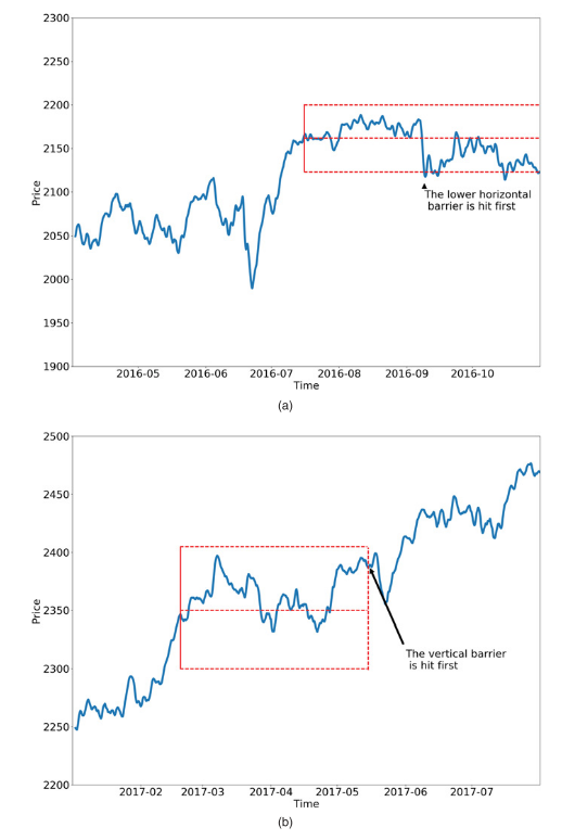
At a given time stamp, 3 barriers are set. An upper and lower horizontal barrier to represent a take profit and stop loss levels. A third and vertical barrier is placed to represent the end of the duration of the trade.

Should the path of a stock reach the upper barrier before the vertical then a value of 1 is returned, conversely if it reaches the bottom barrier then a -1, however should the stock price reach the vertical barrier first then a 0 is returned. This is still a {-1. 0, 1} scheme, however we are labeling a path of returns rather than the next directional move.

The horizontal barriers are determined by calculating the daily standard deviation of the log returns multiplied by a user defined multiple. For example a [1, 1] tuple will set both barriers to be equal to 1 standard deviation.

The following figure provides an example:

An example of Triple-Barrier Labeling from Advances in Financial Machine Learning

Figure 3: Triple Barrier Labeling (Lopez de Prado 2018)

In chart (a) we can see that the lower horizontal barrier is first reached, a -1 value is returned. In chart (b) the path never reaches the horizontal barriers and triggers a 0 label when the vertical barrier is reached.

3.5. Fitting a Primary Model

The primary model is the component that determines which side of the trade to take. It generates a signal {-1, 0, 1}. Where -1 is a short position, 1 is a long position, and 0 means to close all positions.

This model could be but not limited to:

Statistical arbitrage model based on the spread between two assets.
Machine learning model such as an SVM or Neural Network.
Fundamental value or events based strategy where the portfolio manager generates the signal.
Rules based, technical trading strategy such as moving average crossovers.

The only requirement is that a signal is generated which is used to determine the side of the position. We look to meta labeling and bet sizing to determine the size of the position.

The following two sections discuss the technical analysis inspired strategies we used.

3.5.1. Trend Following

A simple moving average crossover strategy is employed. The idea behind this strategy is to make use of two moving averages to help smooth out the noise in the data and then determine when a trend is in affect.

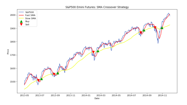
Traditionally a slow 200 day and a fast 50 day moving average are used. When the fast moving average crosses above the slow, a buy signal (1) is generated. Conversely when the fast crosses below the slow then a sell signal (-1) is generated. Under this scheme, there is always a long or a short side active, i.e. no 0 signals. The figure below shows an example of this.

Illustration of the Trend Following Strategy

Figure 4: SMA Crossover Strategy

The green upward arrows indicate when a long (buy) signal is in affect and a red downward arrow a short (sell) signal.

For the primary trend following model we implemented a 20 and 50 bar SMA crossover strategy. Remember that we reduced the number of events by making use of the CUSUM filter, because of this we need much shorter SMA periods to capture the short term trends that may be in affect, and provide more current information to the secondary model since the vertical barrier is set to a single day.

3.5.3. Mean Reversion

The second primary model is based on mean reversion and makes use of Bollinger Bands. Bollinger Bands are a technical analysis indicator which creates bands around the price level which are more than x standard deviations away, where x is a user defined multiple.

The principal is that stock prices are log normally distributed and thus we can make use of the Empirical rule which states that 99.7% of the data lies within 3 standard deviations, 95% within 2 and 68% within 1 standard deviation. Should the closing price be above say 2 standard deviations then we generate short signal (-1) on the premise that prices should mean revert in the near term. The reverse is also true, if prices are below 2 standard deviations a buy signal is generated (1).

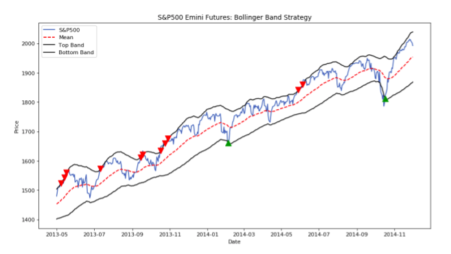
The figure below shows an example of a traditional Bollinger band strategy.

Illustration of the Mean Reverting Strategy

Figure 5: Bollinger Band Mean Reversion Strategy

The green upward arrows indicate when a long (buy) signal is in affect and a red downward arrow a short (sell) signal.

Typically a position is held until the price reaches the moving average but in our case, because we are using the triple barrier method, a position is held until one of the three barriers are touched.

3.6. Meta Labeling

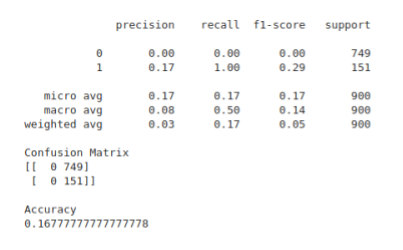
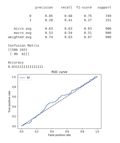
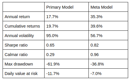
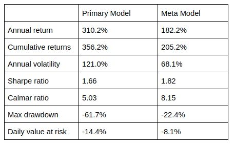
The central idea is to create a secondary machine learning (ML) model that learns how to use the primary exogenous model. This leads to improved performance metrics, including: Accuracy, Precision, Recall, and F1-Score. For those readers who are interested in building up a deeper intuition around meta-labeling, the following blog post illustrates a toy example. We would like to stress the importance of this concept and see it as a major contribution of Dr Lopez de Prado work.

Use in Financial Machine Learning

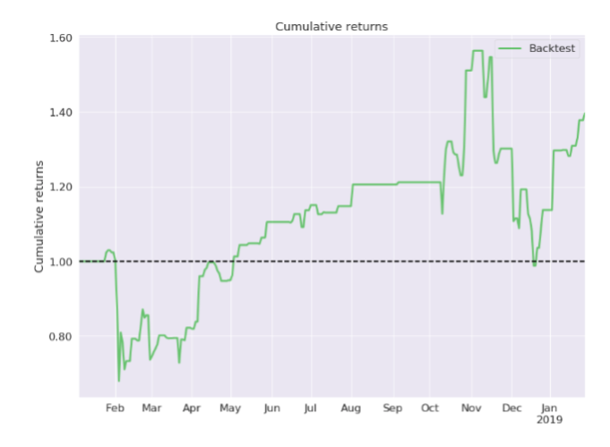
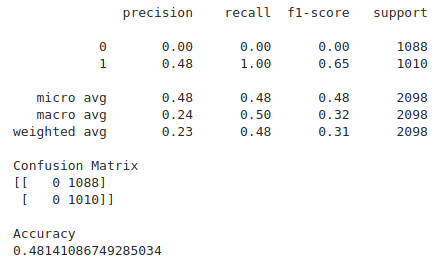
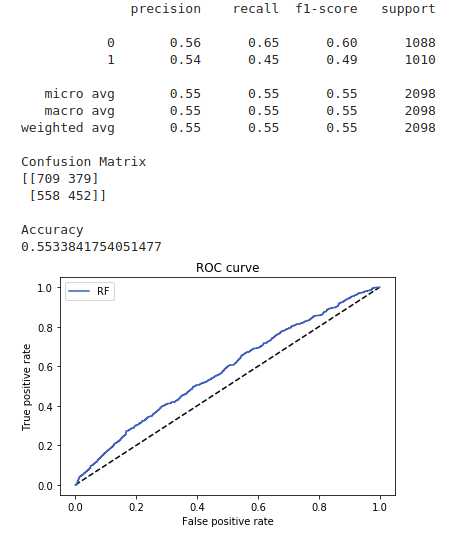
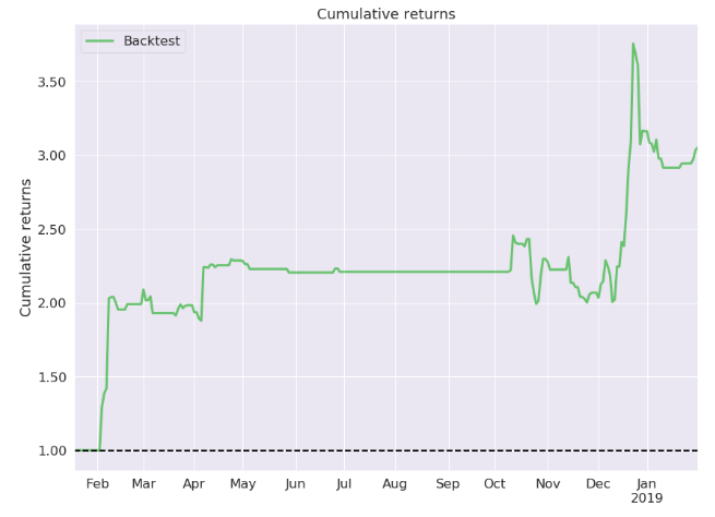
Meta labeling in finance follows the same principles as we outlined in the toy example on the MNIST dataset. First we make use of a primary model, in this case a simple trend following or mean reverting strategy, to determine the position of the trade. Then we fit a Random Forest meta-label model to the primary model to determine when to trade or not.

4. Results

We developed the packages and Jupyter Notebooks and shared them on Github. The core functionality is under the package name “mlfinlab”. As we stated above (in the section, Methodology) that our goal was to build a platform where practitioners can use our codes and also contribute to this research. We are happy to report that this library has received considerable interest from the quantitative finance community and several have volunteered to add to the code base. A few have forked from the repository to extend the work we have done so far.

Screen shot of the Hudson and Thames Github repo

Figure 6: Project Dashboard

4.1. Performance of the Strategies

We tested two trading strategies – trend-following and Bollinger band mean-reverting to use our framework and test their performance. During the training and validation phases of the strategy build-out, we manually tuned a few parameters to ensure that we have sufficient data points. For instance, a function called get_t_events filters the data (using CUSUM filter) for events when there has been a structure shift. We changed the threshold parameter manually to get sufficiently large data set. Second, we found that meta-labeling often resulted in unbalanced classes – to trade (=1) or not to trade (=0) with many more instances of “not to trade”. We used up-sampling to balance these classes prior to training the machine-learning algorithm (Random Forest).

4.1.1 Performance Metrics

To evaluate the efficacy of meta-labeling we look at a models performance metrics between the validation set and the out-of-sample test set. This allows us to draw conclusions about the model’s ability to generalize. In particular we need to look at the recall, precision, F1 score, and accuracy.

The reason why we don’t compare the strategies performance metrics (annualized returns, sharpe ratio, and drawdowns) is because the two data sets are from very different time periods. For example, if the validation set has a much higher volatility than the test set, then the validation returns will be larger. This will prevent like for like comparison.

We can however compare strategy metrics if they are both from the same time period. We do provide performance metrics on the test data. Additionally we add a performance tear sheet, and see that meta-labeling results in better strategy metrics but it should be noted that we have yet to add a bet sizing component to the strategy. Additionally the two strategies we test are based on technical analysis and they don’t provide the best signals. A primary model with better predictive power would provide further insights.

4.1.2. Bollinger Band Mean-Reversion Strategy

We construct 1.5 standard deviation upper and lower bands around the average closing price of the S&P500 e-mini futures. The strategy buys when the close price falls at or below the lower band and sells when the close price rises at or above the upper band. These generate the buy/sell signals also called the “side”. The meta-labeling function decides on the size (to trade or not to trade). This information along with features such as 14-day RSI, volatility, 7 and 15-day moving averages, one to five day auto-correlation, and one to five day momentum is used to train Random Forest algorithm. The trained algorithm is used to validate the signal. Finally, after finalizing the algorithm we use the trained model to test out-of-sample.

The results are as follows:

Validation Data

Figure 7: Primary Model on Validation Set (Mean Reverting)

Meta labeling tearsheet on validation data: Mean Reversion Strategy

Figure 8: Meta Model on Validation Set (Mean Reverting)

In the validation data we can see that the performance metrics increase. The accuracy jumps from 20% to 77%. The precision of correct trades also jumps from 0.21 to 0.39, this will correlate to greater profits and lower drawdowns.

Out-of-Sample Data

Figure 9: Primary Model on Out-of-Sample Set (Mean Reverting)

Meta labeling tearsheet on out of sample data: Mean Reversion Strategy

Figure 10: Meta Model on Out-of-Sample Set (Mean Reverting)

This test data is completely out-of-sample. The precision jumps from 0.17 to 0.20 and the accuracy from 17% to 63%. This should translate to improved strategy performance metrics as well.

Strategy Performance Metrics

Comparison of meta labeling vs the primary model for mean reversion strategy

Table 1: Out-of-sample (2018-01-04 : 2019-01-28)

This shows that the meta-model adds a lot of value to the out-of-sample performance. All the metrics have improved across the board.

Performance Tear Sheet

The following charts are added for sake of completeness and to illustrate the risk return profile of the mean reverting strategy.

Figure 11: Cumulative Returns (Mean Reverting)

Figure 12: 6 Month Volatility and Sharpe Ratio (Mean Reverting)

Figure 13: Drawdowns and Underwater Plot (Mean Reverting)

4.1.3. Simple Moving Average (SMA) Crossover – Trend Following Strategy

We construct two moving averages. A fast 20 bar SMA and a slow 50 bar SMA around the closing price of the S&P500 e-mini futures.

The strategy buys when the fast SMA is above the slow SMA and sells when the fast SMA is below the slow SMA. These generate the buy/sell signals also called the “side”. The meta-labeling function decides on the size (to trade or not to trade). This information along with features such as fifty, thirty one, and fifteen bar rolling volatility, one to five day auto-correlation, and one to five day momentum is used to train Random Forest algorithm. The trained algorithm is used to validate the signal. Finally, after finalizing the algorithm we use the trained model to test out-of-sample.

The results are as follows:

Validation Data

Figure 14: Primary Model on Validation Set (Trend Following)

Meta labeling on validation set for trend following strategy

Figure 15: Meta Model on Validation Set (Trend Following)

In the validation data we can see that the performance metrics increase. The accuracy jumps from 37% to 56%. The precision of correct trades also increases from 0.37 to 0.42, this will correlate to greater profits and lower drawdowns in the long run.

Out-of-Sample Data

Figure 16: Primary Model on Out-of-Sample Set (Trend Following)

Meta labeling on out of sample set for trend following strategy

Figure 17: Meta Model on Out-of-Sample Set (Trend Following)

This test data is completely out-of-sample. The precision increases from 0.48 to 0.54 and the accuracy from 48% to 55%. This should translate to improved strategy performance metrics as well.

Strategy Performance Metrics

Comparison of meta labeling vs the primary model for trend following strategy

Table 2: Out-of-sample (2018-01-18 : 2019-01-31)

The above is slightly different to the mean reverting strategy as it doesn’t out perform on all the metrics however it does outperform on a risk adjusted basis. This is exactly what meta-labeling sets out to do!

Performance Tear Sheet

The following charts are added for sake of completeness and to illustrate the risk return profile of the trend following strategy.

Figure 18: Cumulative Returns (Trend Following)

Figure 19: 6 Month Volatility and Sharpe Ratio (Trend Following)

Figure 20: Drawdowns and Underwater Plot (Trend Following)

5. Next Steps

We plan to continue to enhance and expand the platform and the mlfinlab package. Specifically, in the short-term:

Use the best-practices of cross-validation (see section on Random Forests, Cross-Validation and Grid Search).
Add position sizing (bet sizing [Lopez de Prado 2018, Chapter 10] and risk management to the strategies. This will provide a much more realistic picture of a strategy’s performance.
Build unit-tests for each of the library functions.
Build a “feature zoo”.
Use new features and a better model to redesign the current trend-following strategy.
Test the strategies with other data such as Euro STOXX index.
Write a paper.

6. Conclusion

This capstone project was conceived as a step toward a larger goal of creating a platform for ongoing quantitative research that (Lopez de Prado 2018) speaks about in the form of meta-strategies. Our goal in this phase of the larger endeavor was to create an open-source package that serves as a foundation and then leverage that to test a couple of trading strategies. We also wanted to use concepts, ideas and theories learnt from courses, projects and papers during the MSFE at WorldQuant University.

Given the interest shown by various quant practitioners and Dr. de Prado, the author of the book “Advances in Financial Machine Learning”, we feel that we are on the right track. We also did not want this to be a purely pedagogical but examine the efficacy of the key concepts like meta-labeling and triple-barrier. Our results on the two strategies – trend-following and mean-reversion – bear that out (See Results section).

But as we stated above, this is only the first step and much work needs to be done. We have discussed in the section Next Steps many of the immediate “to dos”. In the long-term we hope to learn more via the discussion and contribution from others as we continue to contribute.

References

This section is best referenced via the pdf document.

[Ale61] Sidney S. Alexander. “Price Movements in Speculative Markets: Trends or Random Walks”. In: Industrial Management Review 2 (1961), pp. 7–26.
[Ale64] Sidney S. Alexander. “Price Movements in Speculative Markets: Trends or Random Walks, No. 2”. In: Industrial Management Review 5 (1964), pp. 25–46.
[EPO11] David Easley, MARCOS L ́OPEZ DE PRADO, and Maureen O’Hara.“The Volume Clock: Insights into the High-Frequency Paradigm”. In: Journal of Portfolio ManagementCl (2011), pp. 901–921.
[FB66] Eugene F. Fama and Marshall E. Blume. “Filter rules and stock-market trading”. In: Journal of Business39.1 (1966), pp. 226–241.
[Has09] Hastie, Trevor. Tibshirani, Robert. Friedman, Jerome. The Elementsof Statistical Learning. 2009.
[LF14] Marcos Lopez de Prado and Matthew D. Foreman. “A mixture ofGaussians approach to mathematical portfolio oversight: the EF3M algorithm”. In: Quantitative Finance14.5 (2014), pp. 913–930.
[LLC18] Tick Data LLC. Global Futures Trade and Quote Data File Format Document, Version 1.6. 2018.
[Lop18] Marcos Lopez de Prado. Advances in Financial Machine Learning. Wiley, 2018, p. 366.
[LY97] Kin Lam and H.C. Yam. “CUSUM Techniques for Technical Trading in Financial Markets”. In: Financial Engineering and Japanese Markets 4 (1997), pp. 257–274.
[NAT16] NATLAT. Scanning hyperspace: how to tune machine learning mod-els. [Online; accessed March 18, 2019].
[Nor18] Norena, Sebastian.Python Model Tuning Methods Using Cross Validation and Grid Search. [Online; accessed March 18, 2019].
[sci19] scikit learn. Precision and recall. [Online; accessed March 18, 2019].
[Sin19] Singh, Ashutosh. Joubert, Jacques. Capstone1. [Online; accessed March18, 2019]
[TH00] Ane Thierry and Geman Helyette. “Order Flow, Transaction Clock, and Normality of Asset Returns”. In: 55.5 (2000), pp. 2259–2284.
[WC06] Jar-long Wang and Shu-hui Chan. “Stock market trading rule dis-covery using two-layer bias decision tree”. In: Expert Systems with Applications 30.1 (2006), pp. 605–611.
[Wik19] Wikipedia, the free encyclopedia. Precision and recall. [Online; accessed March 18, 2019].