Introduction to Distance Approach in Pairs Trading: Part II
by Joohwan Ko
Join the Reading Group and Community: Stay up to date with the latest developments in Financial Machine Learning!
Introduction
We have discussed Basic Distance Approach in the previous blog post. In this post, we’ll look into one of the advanced methods in the Distance Approach and its differences to the Basic Distance Approach. If you haven’t read the previous blog post, we recommend reading it before you read this post:
Pearson Correlation Approach
So, what is the Pearson Correlation Approach? It is a type of Distance Approach and applies Pearson correlation on return level for identifying pairs. The main concept is similar to the Basic Distance Approach, where pairs are formed with a particular rule, and a portfolio is constructed based on the trading signals of pairs.
![]()
The equation above shows the key concept of the Pearson Correlation Approach, where ![]() is return divergence and
is return divergence and ![]() is the regression coefficient of
is the regression coefficient of ![]() ‘s monthly return on its comover return
‘s monthly return on its comover return ![]() . A portfolio is constructed after sorting stocks in descending order based on their previous month’s return divergence.
. A portfolio is constructed after sorting stocks in descending order based on their previous month’s return divergence.
Portfolio Formation
The main concept of this method is to form pairs using Pearson Correlation. Then how do we form portfolios with these pairs? There are three steps in the Portfolio Formation part.
- Data Preprocessing
- Pairs Portfolio Formation
- Trading Signal Generation
Data Preprocessing
First, we need to split the input data. When the prices of stocks are given as an input, the method split data as follows: price data from year ![]() to year
to year ![]() for pairs portfolio formation and price data in year
for pairs portfolio formation and price data in year ![]() for trading. Besides data split, this method usually manipulates the data for further use. As the method has to compute all of the pairs’ correlation values in the following steps, for
for trading. Besides data split, this method usually manipulates the data for further use. As the method has to compute all of the pairs’ correlation values in the following steps, for ![]() stocks, there are
stocks, there are ![]() correlations to be computed in the formation period. As the number of observations for the correlations grows exponentially with the number of stocks, this estimation is computationally intensive.Therefore, this method uses monthly stock returns data in the formation period (ex. 60 monthly stock returns if the formation period is 5 years). Although this manipulation is not necessary, this step may reduce some unnecessary noises of the input data.
correlations to be computed in the formation period. As the number of observations for the correlations grows exponentially with the number of stocks, this estimation is computationally intensive.Therefore, this method uses monthly stock returns data in the formation period (ex. 60 monthly stock returns if the formation period is 5 years). Although this manipulation is not necessary, this step may reduce some unnecessary noises of the input data.
Pairs Portfolio Formation
In the pairs portfolio formation, we have to find pairs first. For each stock, find ![]() stocks with the highest correlations to the stock. After the pairs are selected for each of the stocks, the pairs portfolio formation needs to be done. This “Portfolio” is not the portfolio we will trade in the end but a benchmark portfolio for each of the stocks. That being said, the portfolio of those
stocks with the highest correlations to the stock. After the pairs are selected for each of the stocks, the pairs portfolio formation needs to be done. This “Portfolio” is not the portfolio we will trade in the end but a benchmark portfolio for each of the stocks. That being said, the portfolio of those ![]() stocks only serves as a benchmark for portfolio sorting in the following steps. So, we are setting the pairs portfolio’s returns as the equal-weighted average returns of the top
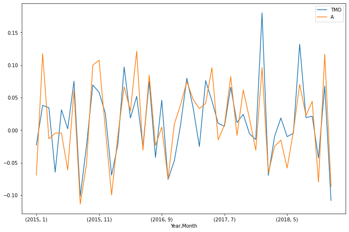
stocks only serves as a benchmark for portfolio sorting in the following steps. So, we are setting the pairs portfolio’s returns as the equal-weighted average returns of the top ![]() pairs of stocks. Below is an example of a pair with a high Perason correlation coefficient.
pairs of stocks. Below is an example of a pair with a high Perason correlation coefficient.
Fig. 1. Plot of two price series of stocks with a high Pearson Correlation.
After pairs portfolios are formed, the method derives ![]() from the monthly return of the stock and its pairs portfolio as follows:
from the monthly return of the stock and its pairs portfolio as follows:
![]()
By using linear regression, setting stock return as independent variable and pairs portfolio return as the dependent variable, the methods set ![]() as a regression coefficient.
as a regression coefficient.
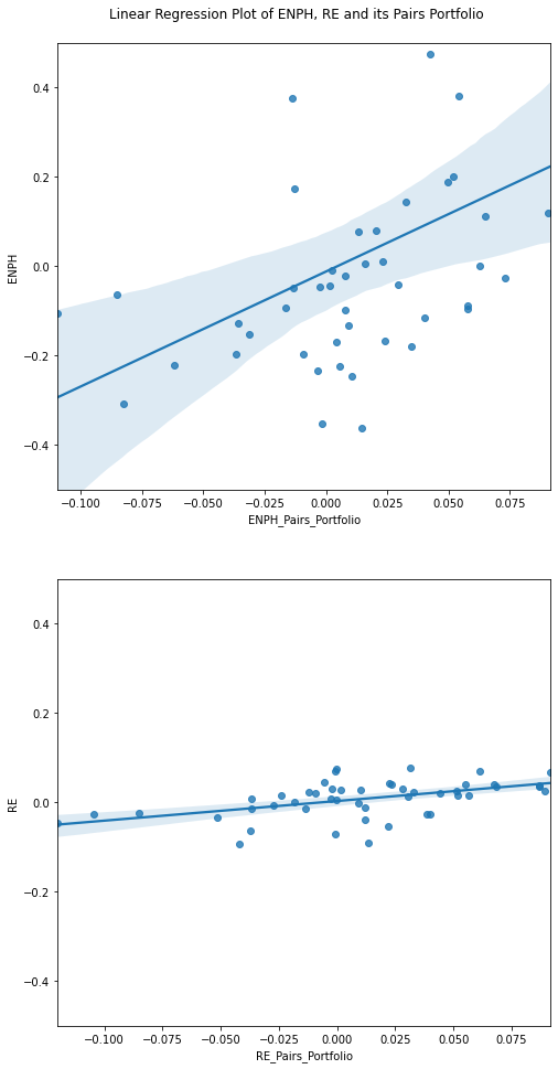
Fig. 2. The first plot shows a stock with a high ![]() and the second plot shows a stock with a low
and the second plot shows a stock with a low ![]() .
.
Trading Signal Generation
The pairwise trading hypothesis is that if a stock’s return deviates from its pairs portfolio returns in any given month in year ![]() , this divergence will be reversed in the following month. The return divergences are calculated with the beta created in the formation period as follows:
, this divergence will be reversed in the following month. The return divergences are calculated with the beta created in the formation period as follows:
![]()
Then, all stocks are sorted in descending order based on their previous month’s return divergence. If the percentages of long/short stocks are given (say 𝑝% and 𝑞%) , the top 𝑝% of the sorted stocks are chosen for the long stocks, and the bottom 𝑞% of the sorted stocks are chosen for the short stocks. A dollar-neutral portfolio can be constructed by longing decile 10 and shorting decile 1, and held for one month.
Differfence to Basic Distance Approach
There are two main differences between the Pearson Approach and Basic Approach.
- Less strict than SSD minimization
- Higher information level contained in a diversified comover portfolio
Less strict than SSD minimization
According to Krauss(2017), let’s take a look at the equation of variance of price spread. In the case of the Basic Distance Approach, we assume that minimizing SSD leads to a minimization of price spread variance. The variance of the spread price reaches its minimum of zero if the two stock prices are perfectly correlated and their price time series exhibit the same variance. Therefore, the minimum SSD criterion thus finds asset prices with similar variance and high correlation.
![]()
On the other hand, if we look at the equation of variance of return spread, constraining for high return correlation leads to lower variance of spread returns. However, the returns of the individual assets may still exhibit different variances.
![]()
Higher information level contained in a diversified comover portfolio
Return divergences from such a portfolio are more likely to be caused by idiosyncratic movements of ![]() , and thus potentially reversible. This hypothesis was tested by Perlin(2007, 2009) that there are advantages of quasi-multivariate pairs trading versus univariate pairs trading. Quasi-multivariate pairs trading results in higher and more robust annual excess returns than univariate pairs trading for a broad range of different threshold values.
, and thus potentially reversible. This hypothesis was tested by Perlin(2007, 2009) that there are advantages of quasi-multivariate pairs trading versus univariate pairs trading. Quasi-multivariate pairs trading results in higher and more robust annual excess returns than univariate pairs trading for a broad range of different threshold values.
Possible Improvements
There are still some limitations of this approach and can be improved in various ways. Below are some examples of them:
- Two assets correlated on return level do not necessarily share an equilibrium relationship.
- As there is no theoretical foundation that divergences need to be reversed divergence reversion needs to be further tested.
- One may add a cointegration test to the selected pairs.
Check out our lecture on the topic:
References
- Krauss, C., 2017. Statistical arbitrage pairs trading strategies: Review and outlook. Journal of Economic Surveys, 31(2), pp.513-545.
- Gatev, E., Goetzmann, W.N. and Rouwenhorst, K.G., 2006. Pairs trading: Performance of a relative-value arbitrage rule. The Review of Financial Studies, 19(3), pp.797-827.
- Do, B. and Faff, R., 2010. Does simple pairs trading still work?. Financial Analysts Journal, 66(4), pp.83-95.
- Do, B. and Faff, R., 2012. Are Pairs Trading Profits Robust to Trading Costs?. SSRN Electronic Journal.
- Perlin, M.S., 2009. Evaluation of pairs-trading strategy at the Brazilian financial market. Journal of Derivatives & Hedge Funds, 15(2), pp.122-136.
- Chen, H., Chen, S., Chen, Z. and Li, F., 2019. Empirical investigation of an equity pairs trading strategy. Management Science, 65(1), pp.370-389.
- Perlin, M. (2007). M of a Kind: A Multivariate Approach at Pairs Trading. SSRN Electronic Journal.


