Portfolio Optimisation with PortfolioLab: Estimation of Risk
By IIlya Barziy, Aman Dhaliwal and Aditya Vyas
Join the Reading Group and Community: Stay up to date with the latest developments in Financial Machine Learning!

Risk has always played a very large role in the world of finance with the performance of a large number of investment and trading strategies being dependent on the efficient estimation of underlying market risk. With regards to this, one of the most popular and commonly used representation of risk in finance is through a covariance matrix – higher covariance values mean more volatility in the markets and vice-versa. This also comes with a caveat – empirical covariance values are always measured using historical data and are extremely sensitive to small changes in market conditions. This makes the covariance matrix an unreliable estimator of the true risk and calls for a need to have better estimators.
In this post we will use the RiskEstimators class from PortfolioLab which provides several implementations for different ways to calculate and adjust the empirical covariance matrices. Some of these try to remove inherent outliers from the matrix while others focus on removing noise from the empirical values. Throughout this blog post, we will look at a quick description of each algorithm as well as see how we can use the corresponding implementation provided in PortfolioLab.
The RiskEstimators class covers seven different algorithms relating to covariance matrix estimators. These algorithms include:
- Minimum Covariance Determinant
- Empirical Covariance
- Covariance Estimator with Shrinkage
- Semi-Covariance Matrix
- Exponentially-Weighted Covariance matrix
- De-Noising Covariance Matrix
- Covariance and Correlation Matrix Transformations
Note: The descriptions of these algorithms are all based upon the descriptions from the scikit-learn User Guide on Covariance Estimation. Infact, most of the methods (except the denoising and detoning ones) in the class are wrappers of sklearn’s covariance methods but with the added functionality of working specifically with financial data e.g. having inbuilt returns calculation.
We will import the required libraries and the dataset – a small subset of historical prices of ETFs.
# importing our required libraries
import numpy as np
import pandas as pd
import matplotlib.pyplot as plt
import portfoliolab as pl
# reading in our data
stock_prices = pd.read_csv('stock_prices.csv', parse_dates=True, index_col='Date')
stock_prices = stock_prices.dropna(axis=1)
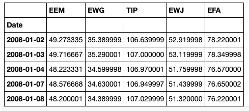
For the purpose of this post, we will only use 5 assets, so the differences between the calculated covariance matrices are easy to see.
stock_prices = stock_prices.iloc[:, :5]
stock_prices.head()
Minimum Covariance Determinant
The Minimum Covariance Determinant (MCD) is a robust estimator of covariance that was introduced by P.J. Rousseeuw. From the scikit-learn User Guide on Covariance Estimation, “the basic idea of the algorithm is to find a set of observations that are not outliers and compute their empirical covariance matrix, which is then rescaled to compensate for the performed selection of observations”. The PortfolioLab implementation is a wrap around sklearn’s MinCovDet class, which uses FastMCD algorithm, developed by Rousseeuw and Van Driessen. A detailed description of the algorithm is available in the paper by Mia Hubert and Michiel Debruyne – Minimum Covariance Determinant.
First, we can construct a simple (empirical) covariance matrix for comparison.
# A class with function to calculate returns from prices
returns_estimation = pl.estimators.ReturnsEstimators()

# Calcualting the data set of returns
stock_returns = returns_estimation.calculate_returns(stock_prices)

# Finding the simple covariance matrix from a series of returns
cov_matrix = stock_returns.cov()
We can now construct the MCD matrix. One can use minimum_covariance_determinant() method for this purpose.
# A class that has the Minimum Covariance Determinant estimator
risk_estimators = pl.estimators.RiskEstimators()

# Finding the Minimum Covariance Determinant estimator on price data and with set random seed to 0
min_cov_det = risk_estimators.minimum_covariance_determinant(stock_prices, price_data=True, random_state=0)

# Transforming our estimation from a np.array to pd.DataFrame
min_cov_det = pd.DataFrame(min_cov_det, index=cov_matrix.index, columns=cov_matrix.columns)


From the above images, you can see that the absolute values in the Minimum Covariance Determinant estimator are lower in comparison to the simple Covariance matrix, which means that the algorithm has eliminated some of the outliers in the data and the resulting covariance matrix estimator is a more robust one. Note that this method achieves the best result when the data has outliers in it.
Maximum Likelihood Covariance Estimator (Empirical Covariance)
Maximum Likelihood Estimator of a sample is an unbiased estimator of the corresponding population’s covariance matrix. This estimation works well when the number of observations is big enough in relation to the number of features.
We can implement this algorithm through the empirical_covariance method() in the PortfolioLab library.
# Finding the Empirical Covariance on price data
empirical_cov = risk_estimators.empirical_covariance(stock_prices, price_data=True)

# Transforming Empirical Covariance from np.array to pd.DataFrame
empirical_cov = pd.DataFrame(empirical_cov, index=cov_matrix.index, columns=cov_matrix.columns)

One can observe that the Empirical Covariance is the same as the standard covariance function from the pandas package i.e. the cov() function.
Covariance Estimator with Shrinkage
According to the scikit-learn User Guide on Covariance estimation:
“The Maximum Likelihood Estimator is not a good estimator of the eigenvalues of the covariance matrix and the inverted matrix is not accurate. Sometimes, … it cannot be inverted for numerical reasons. To avoid problems with inversion, a transformation of the empirical covariance matrix has been introduced: the shrinkage. Mathematically, this shrinkage consists of reducing the ratio between the smallest and the largest eigenvalues of the empirical covariance matrix”.
There are three different types of shrinkage which we will be looking at in this article. These methods include: Basic Shrinkage, Ledoit-Wolf Shrinkage, and Oracle Approximating Shrinkage.
Basic Shrinkage
Essentially, the Basic Shrinkage method makes use of the following convex transformation: \begin{aligned}\sum_{shrunk} = (1 – \alpha)*\hat{\sum} \: + \: \alpha*\frac{Tr(\hat{\sum})Id}{P}\end{aligned} where  is the empirical covariance matrix and
  represents our trade-off between bias and variance. The definition given by the scikit-learn User Guide on Covariance estimation gives a clear understanding of what this method aims to accomplish:
“This shrinkage is done by shifting every eigenvalue according to a given offset, which is equivalent to finding the l2-penalized Maximum Likelihood Estimator of the covariance matrix”.
In the PortfolioLab implementation, is passed to a function as the basic_shrinkage parameter.
Ledoit-Wolf Shrinkage
The Ledoit-Wolf Shrinkage method differs from the Basic Shrinkage method as it aims to compute the optimal value that minimizes the mean squared error between the estimated and the real covariance matrix.
The algorithm is described in more detail in the paper by Olivier Ledoit and Michael Wolf – A Well-Conditioned Estimator for Large-Dimensional Covariance Matrices.
Oracle Approximating Shrinkage
The Oracle Approximating Shrinkage method works under the assumption that the data we are using falls under a Gaussian distribution. In 2010, Chen et al. derived a formula which chooses the shrinkage coefficient to yield a smaller mean squared error than the one found in the Ledoit-Wolf method.
The algorithm is described in more detail in the paper by Y. Chen, A. Wiesel, Y.C. Eldar and A.O. Hero – Shrinkage Algorithms for MMSE Covariance Estimation.
The shrinked_covariance() method from PortfolioLab allows us to easily calculate the Shrinked Covariances for each of the three methods described above.
# Finding the Shrinked Covariances on price data with every method
shrinked_cov = risk_estimators.shrinked_covariance(stock_prices, price_data=True,
                                                   shrinkage_type='all', basic_shrinkage=0.1)

# Separating the Shrinked covariances for every method
shrinked_cov_basic, shrinked_cov_lw, shrinked_cov_oas = shrinked_cov

# Transforming each Shrinked Covariance from np.array to pd.DataFrame
shrinked_cov_basic = pd.DataFrame(shrinked_cov_basic, index=cov_matrix.index, columns=cov_matrix.columns)
shrinked_cov_lw = pd.DataFrame(shrinked_cov_lw, index=cov_matrix.index, columns=cov_matrix.columns)
shrinked_cov_oas = pd.DataFrame(shrinked_cov_oas, index=cov_matrix.index, columns=cov_matrix.columns)


The Shrinked Covariance matrices for the Ledoit-Wolf and Oracle Approximating algorithms are similar with absolute covariance values in the Oracle Approximating covariance matrix being slightly bigger. With the basic Shrinkage covariance matrix with  , the absolute values are even smaller. The Empirical Covariance matrix has the highest absolute values in comparison.
Semi-Covariance Matrix
Semi-covariance matrix is the way to measure the volatility of the negative returns or returns below a certain threshold.
This measure can be used to decrease negative volatility and is more precise for this goal than the covariance matrix that measures both positive and negative variance. Each element in the Semi-Covariance matrix is calculated as:\begin{aligned}SemiCov_{ij} = \frac{1}{T}\sum_{t=1}^{T}[Min(R_{i,t}-B,0)*Min(R_{j,t}-B,0)] \end{aligned} where  is the number of observations,
  is the return of an asset
  at time
  , and
, and  is the threshold return. If the is set to zero, the volatility of negative returns is measured.
A deeper analysis of use cases of Semi-Covariance matrix is available in the paper by Solactive AG – German Index Engineering – Minimum Downside Volatility Indices.
We can calculate the Semi-Covariance and compare it to the simple/empirical covariance.
# Finding the Semi-Covariance on price data
semi_cov = risk_estimators.semi_covariance(stock_prices, price_data=True, threshold_return=0)

# Transforming Semi-Covariance from np.array to pd.DataFrame
semi_cov = pd.DataFrame(semi_cov, index=cov_matrix.index, columns=cov_matrix.columns)


As the computation of the Semi-Covariance matrix is different from the usual computation of the covariance matrix, the absolute values in the Semi-Covariance matrix are significantly lower. Since it’s a measure, let’s multiply the Semi-Covariance matrix by 10 to better see the changes in the measures.
semi_cov * 10
Now we can see that the values in the two matrices are similar, however, some differences are present. For example, the simple Covariance between EEM and TIP is negative, but the negative returns have positive covariance.

Exponentially-Weighted Covariance Matrix
Each element in the Exponentially-weighted Covariance matrix is calculated as follows.
First, we calculate the series of covariances for every observation time between two elements and  , \begin{aligned}CovarSeries_{i,j}^{t} = (R_{i}^{t} – Mean(R_{i})) * (R_{j}^{t} – Mean(R_{j})) \end{aligned} Then we apply the exponential weighted moving average based on the obtained series with decay in terms of span, as
  \begin{aligned}ExponentialCovariance_{i,j} = EWMA(CovarSeries_{i,j})[T]\end{aligned} where
  refers to Exponentially Weighted Moving Average.
So, it’s the last element from an exponentially weighted moving average series based on a series of covariances between returns of the corresponding assets. It is used to give greater weight to most recent observations in computing the covariance.
We can calculate the Exponential Covariance and compare it to the simple covariance.
exponential_cov = risk_estimators.exponential_covariance(stock_prices, price_data=True, window_span=60)

# Transforming Semi-Covariance from np.array to pd.DataFrame
exponential_cov = pd.DataFrame(exponential_cov, index=cov_matrix.index, columns=cov_matrix.columns)


De-Noising Covariance Matrix
The main idea behind de-noising the covariance matrix is to eliminate the eigenvalues of the covariance matrix that are representing noise and not useful information.
Constant Residual Eigenvalue De-noising Method
This is done by determining the maximum theoretical value of the eigenvalue of such matrix as a threshold and then setting all the calculated eigenvalues above the threshold to the same value.
The function provided below for de-noising the covariance works as follows:
- The given covariance matrix is transformed to the correlation matrix.
- The eigenvalues and eigenvectors of the correlation matrix are calculated.
- Using the Kernel Density Estimate algorithm a kernel of the eigenvalues is estimated.
- The Marcenko-Pastur pdf is fitted to the KDE estimate using the variance as the parameter for the optimization.
- From the obtained Marcenko-Pastur distribution, the maximum theoretical eigenvalue is calculated using the formula in the section Instability caused by noise in the following paper – A Robust Estimator of the Efficient Frontier.
- The eigenvalues in the set that are above the theoretical value are all set to their average value. For example, we have a set of 5 sorted eigenvalues
 two of which are above the maximum theoretical value, then we set \begin{aligned}\lambda^{NEW}_{4} = \lambda^{NEW}_{5} = \frac{\lambda^{OLD}_{4} + \lambda^{OLD}_{5}}{2}\end{aligned}
 - Eigenvalues above the maximum theoretical value are left intact. \begin{aligned}\lambda^{NEW}_{1} = \lambda^{OLD}_{1}\end{aligned} \begin{aligned}\lambda^{NEW}_{2} = \lambda^{OLD}_{2}\end{aligned} \begin{aligned}\lambda^{NEW}_{3} = \lambda^{OLD}_{3}\end{aligned}
- The new set of eigenvalues with the set of eigenvectors is used to obtain the new de-noised correlation matrix.
 is the de-noised correlation matrix,
  is the eigenvectors matrix, and
  is the diagonal matrix with new eigenvalues.
 - The new correlation matrix is then transformed back to the new de-noised covariance matrix.\begin{aligned}\tilde{C} = W \Lambda W\end{aligned}
- To rescale $\tilde{C}$ so that the main diagonal consists of 1s the following transformation is made. This is how the final $C_{denoised}$ is obtained.\begin{aligned}C_{denoised} = \tilde{C} [(diag[\tilde{C}])^\frac{1}{2}(diag[\tilde{C}])^{\frac{1}{2}’}]^{-1}\end{aligned}
- The new correlation matrix is then transformed back to the new de-noised covariance matrix.
The process of de-noising the covariance matrix is described in a paper by Potter M., J.P. Bouchaud, L. Laloux – Financial Applications of Random Matrix Theory: Old Laces and New Pieces.
# Setting the required parameters for de-noising

# Relation of number of observations T to the number of variables N (T/N)
tn_relation = stock_prices.shape[0] / stock_prices.shape[1]

# The bandwidth of the KDE kernel
kde_bwidth = 0.25

# Finding the Вe-noised Сovariance matrix
cov_matrix_denoised = risk_estimators.denoise_covariance(cov_matrix, tn_relation, kde_bwidth)

# Transforming De-noised Covariance from np.array to pd.DataFrame
cov_matrix_denoised = pd.DataFrame(cov_matrix_denoised, index=cov_matrix.index, columns=cov_matrix.columns)


As we can see, the main diagonal hasn’t changed, but the other covariances are different. This means that the algorithm has affected those eigenvalues of the correlation matrix which have more noise associated with them.
Targeted Shrinkage De-noising Method
PortfolioLab also has the Targeted Shrinkage De-noising method available to users. The main idea is to shrink the eigenvectors/eigenvalues that are noise-related.This is done by shrinking the correlation matrix calculated from noise-related eigenvectors/eigenvalues and then adding the correlation matrix composed from signal-related eigenvectors/eigenvalues.
The de-noising function works as follows:
- The given covariance matrix is transformed to the correlation matrix.
- The eigenvalues and eigenvectors of the correlation matrix are calculated and sorted in the descending order.
- Using the Kernel Density Estimate algorithm a kernel of the eigenvalues is estimated.
- The Marcenko-Pastur pdf is fitted to the KDE estimate using the variance as the parameter for the optimization.
- From the obtained Marcenko-Pastur distribution, the maximum theoretical eigenvalue is calculated using the formula from the section Instability caused by noise in the paper – A Robust Estimator of the Efficient Frontier.
- The correlation matrix composed from eigenvectors and eigenvalues related to noise (eigenvalues below the maximum theoretical eigenvalue) is shrunk using the variable. \begin{aligned}C_n = \alpha W_n \Lambda_n W_n’ + (1 – \alpha) diag[W_n \Lambda_n W_n’]\end{aligned}
- The shrinked noise correlation matrix is summed to the information correlation matrix.\begin{aligned}C_i = W_i \Lambda_i W_i’\end{aligned}\begin{aligned}C_{denoised} = C_n + C_i\end{aligned}
- The new correlation matrix is then transformed back to the new de-noised covariance matrix.
We can use this method by setting the denoise_method parameter to ‘target_shrink’.
# Relation of number of observations T to the number of variables N (T/N)
tn_relation = stock_prices.shape[0] / stock_prices.shape[1]

# The bandwidth of the KDE kernel
kde_bwidth = 0.01

# Finding the De-noised Сovariance matrix using the Targeted Shrinkage Method assuming alpha is 0.5
cov_matrix_target_denoised = risk_estimators.denoise_covariance(cov_matrix, tn_relation, denoise_method='target_shrink', kde_bwidth=kde_bwidth, alpha=0.5)

# Transforming De-noised Covariance from np.array to pd.DataFrame
cov_matrix_target_denoised = pd.DataFrame(cov_matrix_denoised, index=cov_matrix.index, columns=cov_matrix.columns)


The results of this de-noising method are the same as for the previous method for this particular example, however, they may differ when used on other datasets.
Detoning
De-noised correlation matrix from the previous methods can also be de-toned by excluding a number of first
eigenvectors representing the market component. According to Prof. Marcos Lopez de Prado:
“Financial correlation matrices usually incorporate a market component. The market component is characterized by the first eigenvector, with loadings  Accordingly, a market component affects every item of the covariance matrix. In the context of clustering applications, it is useful to remove the market component, if it exists (a hypothesis that can be tested statistically). By removing the market component, we allow a greater portion of the correlation to be explained by components that affect specific subsets of the securities. It is similar to removing a loud tone that prevents us from hearing other sounds. The detoned correlation matrix is singular, as a result of eliminating (at least) one eigenvector. This is not a problem for clustering applications, as most approaches do not require the invertibility of the correlation matrix. Still, a detoned correlation matrix
  cannot be used directly for mean-variance portfolio optimization”
The de-toning function works as follows:
- De-toning is applied on the de-noised correlation matrix.
- The correlation matrix representing the market component is calculated from market component eigenvectors and eigenvalues and then subtracted from the de-noised correlation matrix. This way the de-toned correlation matrix is obtained.\begin{aligned}\hat{C} = C_{denoised} – W_m \Lambda_m W_m’\end{aligned}
- De-toned correlation matrix
 is then rescaled so that the main diagonal consists of 1s\begin{aligned}C_{detoned} = \hat{C} [(diag[\hat{C}])^\frac{1}{2}(diag[\hat{C}])^{\frac{1}{2}’}]^{-1}\end{aligned}
One can apply de-toning to the covariance matrix by setting the detone parameter to True, as shown in the following snippet. Note that detoning will always be used with either of the denoising methods described before.
# Finding the De-toned Сovariance matrix assuming the market component is 1
cov_matrix_detoned = risk_estimators.denoise_covariance(cov_matrix, tn_relation, denoise_method='const_resid_eigen',
                                                        detone=True, market_component=1,kde_bwidth=kde_bwidth)

# Transforming De-noised Covariance from np.array to pd.DataFrame
cov_matrix_detoned = pd.DataFrame(cov_matrix_detoned, index=cov_matrix.index, columns=cov_matrix.columns)


The results of de-toning are significantly different from the de-noising results. This indicates that the deleted market component had an effect on the covariance between elements.
Covariance and Correlation Matrix Transformations
Additionally, the RiskEstimators class also provides simple utility functions to:
- transform covariance matrix into correlation matrix
- transform correlation matrix into covariance matrix
# Transforming our covariance matrix to a correlation matrix
corr_matrix = risk_estimators.cov_to_corr(cov_matrix)

# The standard deviation to use when calculating the covaraince matrix back
std = np.diag(cov_matrix) ** (1/2)

# And back to the covariance matrix
cov_matrix_again = risk_estimators.corr_to_cov(corr_matrix, std)
Conclusion and Further Reading
This post was intended as a quick introduction to the different ways of adjusting the covariance matrix and produce better and reliable risk estimators. Some important takeaways from the post:
- A robust covariance estimator (such as the Minimum Covariance Determinant) is needed in order to discard/downweight the outliers in the data. The Empirical covariance estimator is extremely sensitive to these outliers and can result in inefficient estimation of risk.
- The Maximum Likelihood Estimator (Empirical Covariance) of a sample is an unbiased estimator of the corresponding population’s covariance matrix.
- Shrinkage consists of reducing the ratio between the smallest and the largest eigenvalues of the empirical covariance matrix. It is used to avoid the problem with inversion of the covariance matrix.
- Ledoit-Wolf and Oracle Approximating are methods to calculate the optimal shrinkage coefficient used in the Basic Shrinkage.
- The semi-covariance matrix is the way to measure the volatility of the negative returns or returns below a certain threshold.
- Exponential Covariance is used to give greater weight to the most relevant observations in computing the covariance.
- The De-noising algorithm calculates the eigenvalues of the correlation matrix and eliminates the ones that are higher than the theoretically estimated ones, as they are induced by noise.
Finally, one should always use these methods appropriately and with caution. Each of these methods are suited to particular objectives e.g. removing outliers, shrinking the eigenvalues, placing more emphasis on relevant observations etc… and no single one is the best of them. If you want to delve deeper into the theory of these algorithms, here is a list of some good reading articles, research papers and notebooks.

