Portfolio Optimisation with PortfolioLab: Theory-Implied Correlation Matrix
By IIlya Barziy, Aman Dhaliwal and Aditya Vyas
Join the Reading Group and Community: Stay up to date with the latest developments in Financial Machine Learning!

Traditionally, correlation matrices have always played a large role in finance. They have been used in tasks ranging from portfolio management to risk management and are calculated based on historical empirical observations. Although they are used so frequently, these correlation matrices often have poor predictive power and prove to be unreliable estimators. Additionally, there are also factor-based correlation matrices, which also do not perform well due to their non-hierarchical structure.
In a 2019 paper written by Marcos López de Prado, he introduced the Theory-Implied Correlation (TIC) algorithm. It demonstrated a new machine learning approach to estimate correlation matrices based on economic theory, rather than historical observations or being factor-based. The TIC algorithm estimates a forward-looking correlation matrix implied by a proposed hierarchical structure of the assets and is computed in three main steps:
- Fitting our tree graph structure based on the empirical correlation matrix
- Deriving our correlation matrix from the linkage object
- De-noising the correlation matrix
Today, we will be exploring the TIC algorithm and look at how to leverage PortfolioLab’s implementation of the same.
How the TIC algorithm works?
In this section, we will be going through a quick summary of the steps involved in computing the TIC matrix.
Fitting our Tree Graph Structure
In this algorithm, the tree graph represents the economic theory and hierarchical structure of our assets. This tree structure is fit based upon our empirical correlation matrix. Essentially, this structure will tell us which assets are closely related to each other and the relative distance between them. This results in a binary tree using an agglomerative clustering technique which can be visualized through a dendrogram. However, this is not the final tree graph we are looking for. The dendrogram always has two items per cluster while our actual tree graph could have one or more leaves per branch. Additionally, the dendrogam will always have clusters while the tree graph may have an unlimited number of levels and our dendrogram incorporates the notion of distance but the tree graph does not.
The general steps for this part of the algorithm are as follows:
- If there is no top level of the tree (tree root), this level is added so that all variables are included in one general cluster.
- The empirical correlation matrix is transformed into a matrix of distances using the above formula:\begin{aligned}d(i, j) = \sqrt{0.5 * (1 – \rho(i,j))}\end{aligned}
- For each level of the tree, the elements are grouped by elements from the higher level. The algorithm iterates from the lowest to the highest level of the tree.
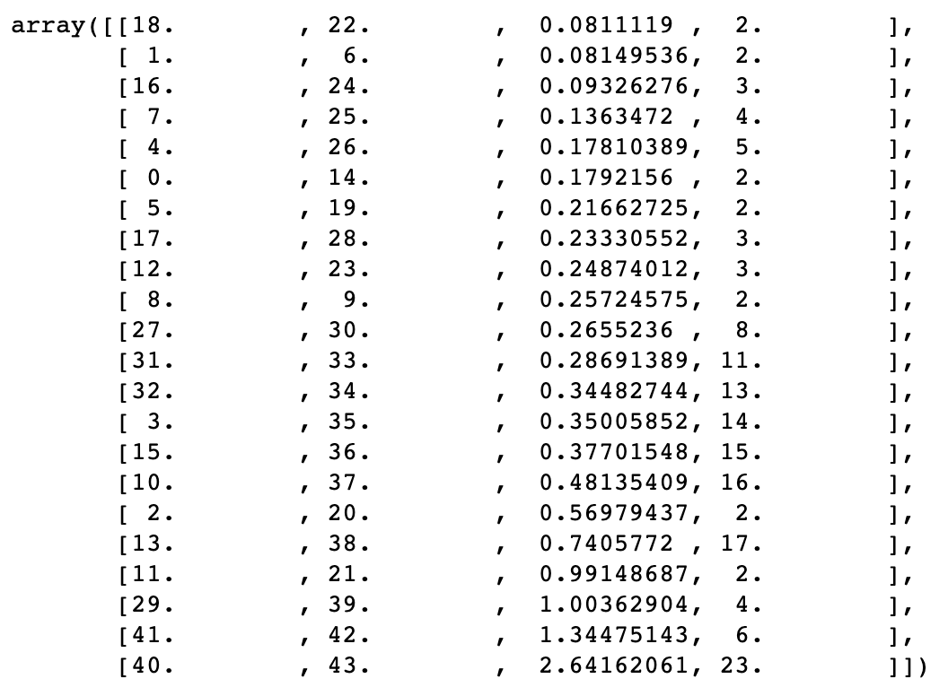
- A linkage object is created for these grouped elements based on their distance matrix. Each link in the linkage object is an array representing a cluster of two elements and has the following data as elements.
- ID of the first element in a cluster
- ID of the second element in a cluster
- Distance between the elements
- Number of atoms (simple elements from the portfolio and not clusters) inside
- A linkage object is transformed to reflect the previously created clusters.
- A transformed local linkage object is added to the global linkage object.
- Distance matrix is adjusted to the newly created clusters – elements that are now in the new clusters are replaced by the clusters in the distance matrix. The distance from the new clusters to the rest of the elements in the distance matrix is calculated as a weighted average of distances of two elements in a cluster to the other elements. The weight is the number of atoms in an element. So, the formula is:\begin{aligned}DistanceCluster = \frac{Distance_{1}*NumAtoms_{1} + Distance_{2}*NumAtoms_{2}}{NumAtoms_{1} + NumAtoms_{2}}\end{aligned}
The linkage object, representing a dendrogram of all elements in a portfolio is the result of the first step of the algorithm. It sequentially clusters two elements together, while measuring how closely together the two elements are, until all elements are subsumed within the same cluster. The final object looks something like this:
Deriving the Correlation Matrix
We can now derive a correlation matrix from our linkage object returned by the first step.
- One by one, the clusters (each represented by a link in the linkage object) are decomposed to lists of atoms contained in each of the two elements of the cluster.
- The elements on the main diagonal of the resulting correlation matrix are set to 1s. The off-diagonal correlations between the variables are computed as:\begin{aligned}\rho(i, j) = 1 – 2*d^{2}(i, j)\end{aligned}
De-Noising the Correlation Matrix
In our last step, the correlation matrix is de-noised.
- The eigenvalues and eigenvectors of the correlation matrix are calculated.
- Marcenko-Pastur distribution is fit to the eigenvalues of the correlation matrix and the maximum theoretical eigenvalue is calculated.
- This maximum theoretical eigenvalue is set as a threshold and all the eigenvalues above the threshold are shrinked.
- The de-noised correlation matrix is calculated back from the eigenvectors and the new eigenvalues.
Using PortfolioLab’s TIC Implementation
In this section, we will go through a working example of using the TIC implementation provided by PortfolioLab and test it on a portfolio of assets.
import portfoliolab as pl
import numpy as np
import pandas as pd
import seaborn as sns
import matplotlib.pyplot as plt
Specifying the Economic Structure a.k.a Tree Graph
The TIC algorithm combines both an economic theory and empirical data. The economic theory is represented by a tree graph and our empirical data is represented by an empirical correlation matrix.
As mentioned previously, the tree graph embeds important information about the hierarchy of the assets in our portfolio and this comes from external market knowledge. Let us look at how to create the graph file.
An example of a hierarchical structure for the financial instruments is the MSCI’s Global Industry Classification Standard (GICS) that classifies investment universes in terms of four nested levels – sub-industry, industry, industry group, and sector. Investors can also add more diverse levels in the tree such as business ties, supply chain, competitors, industrial sectors, shared ownership, etc… For this blog post, we are using a dataset of ETFs and have created an example dataframe representing the tree graph:
# Getting the tree graph for ETFs
etf_tree = pd.read_csv("classification_tree.csv")

# Having a loot at the tree structure of ETFs
print(etf_tree)
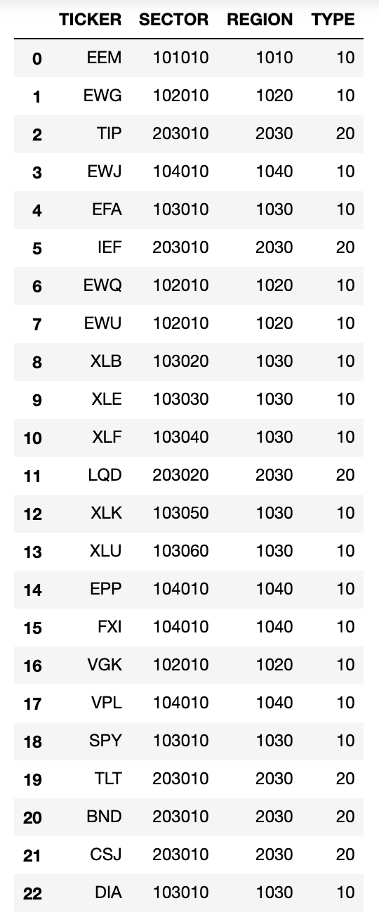
The proposed tree structure has four levels:
- Ticker of the ETF
- Sector of the ETF
- XXXX10 – General/No sector
- XXXX20 – Materials
- XXXX30 – Energy
- XXXX40 – Financial
- XXXX50 – Technology
- XXXX60 – Utilities
- Region of the ETF
- XX10 – Emerging markets
- XX20 – Europe
- XX30 – US and Canada
- XX40 – Asia
- Type of the ETF
- 10 – Equity ETF
- 20 – Bond ETF
The columns are ordered bottom-up, with the leftmost column corresponding to the terminal leaves, and the rightmost column corresponding to the tree’s root. This means that if you converted this dataframe into a tree, then the topmost level would be the type of the asset (in this case, ETF) with the subsequent nested levels being region, sector and finally the asset itself.
Calculating the Empirical Correlation Matrix
Now we calculate the series of returns from the raw prices and finally get the empirical correlations.
# Getting the price data for ETFs
etf_prices = pd.read_csv('stock_prices.csv', parse_dates=True, index_col='Date')

# Class with returns calculation function
ret_est = pl.estimators.ReturnsEstimators()

# Calculating returns
etf_returns = ret_est.calculate_returns(etf_prices)

# Now the emperical correlation matrix can be calculated
etf_corr = etf_returns.corr()
Calculating the TIC Matrix
Equipped with the tree graph and the empirical correlation matrix, we merge them using the TIC algorithm to generate the new correlation matrix.
# Calculating the relation of sample length T to the number of variables N
# It's used for de-noising the TIC matrix
tn_relation = etf_returns.shape[0] / etf_returns.shape[1]

# Class with TIC function
tic = pl.estimators.TheoryImpliedCorrelation()

# Calculating theory-implied correlation matrix
etf_tic = tic.tic_correlation(etf_tree, etf_corr, tn_relation)

# Setting the indexes of the theory-implied correlation matrix
etf_tic = pd.DataFrame(etf_tic, index=etf_corr.index, columns=etf_corr.index)
Visualising the TIC Matrix
We can visualize the difference between the Empirical correlation matrix and the Theory-implied correlation matrix using heatmaps.
# Plotting the heatmap of the matrix
sns.heatmap(etf_corr, cmap="Greens")
plt.title('Empirical Correlation Matrix')
plt.show()

sns.heatmap(etf_tic, cmap="Greens")
plt.title('Theory-Implied Correlation Matrix')
plt.show()


One can observe that the TIC matrix is less noisy and is more smoother. The external market views are incorporated into the empirical values to adjust the noise and get better estimates of the underlying correlations.
However, you might be wondering – if there is such a large visible difference between the two matrices, can we trust the new correlations? Does the TIC algorithm remove much more than just noise and lead to loss of the true correlations between the assets?. One can test the similarity of the two matrices using the correlation matrix distance introduced by Herdin and Bonek in a paper AMIMO Correlation Matrix based Metric for Characterizing Non-Stationarity available here.
# Calculating the correlation matrix distance
distance = tic.corr_dist(etf_corr, etf_tic)

# Printing the result
print('The distance between empirical and the theory-implied correlation matrices is' , distance)
The distance between empirical and the theory-implied correlation matrices is 0.035661302090136404
The correlation matrices are different but are not too far apart. This shows that the theory-implied correlation matrix blended theory-implied views with empirical ones.
You can see that the dendrograms generated from the respective correlation matrices are also visibly different from each other. The TIC dendrogram structure appears to be less complex and a simple hierarchy as compared to the empirical one.


Conclusion and Further Reading
Throughout this tutorial post, we learned about the intuition behind the Theory-Implied Correlation algorithm and how to use PortfolioLab’s implementation of the same. By combining external market views with empirical observations, the TIC algorithm removes the underlying noise from traditional correlation measurements and generates better estimates of the portfolio correlations. Here is an excerpt taken directly from the original paper:
For over half a century, most asset managers have used historical correlation matrices (empirical or factor-based) to develop investment strategies and build diversified portfolios. When financial variables undergo structural breaks, historical correlation matrices do not reflect the correct state of the financial system, hence leading to wrong investment decisions. TIC matrices open the door to the development of forward-looking investment strategies and portfolios.
The following links provide a more detailed exploration of the algorithm and other sources for further reading.

