Portfolio Optimisation with PortfolioLab: Hierarchical Equal Risk Contribution
By Aman Dhaliwal and Aditya Vyas
Join the Reading Group and Community: Stay up to date with the latest developments in Financial Machine Learning!
Harry Markowitz’s Modern Portfolio Theory (MPT) was seen as an amazing accomplishment in portfolio optimization, earning him a Nobel Prize for his work. it is based on the hypothesis that investors can optimize their portfolios based on a given level of risk. While this theory works very well mathematically, it fails to translate to real-world investing. This can be mainly attributed to two different reasons:
- MPT involves the estimation of returns for a given set of assets. Although, accurately estimating returns for a set of assets is very difficult, in which small errors in estimation can cause sub-optimal performance.
- Traditional optimization methods involve the inversion of a covariance matrix for a set of assets. This matrix inversion leads the algorithm to be susceptible to market volatility and can heavily change the results for small changes in the correlations.
In 2016, Dr. Marcos Lopez de Prado introduced an alternative method for portfolio optimization, the Hierarchical Risk Parity (HRP) algorithm. This algorithm introduced the notion of hierarchy and can be computed in three main steps:
- Hierarchical Clustering – breaks down our assets into hierarchical clusters
- Quasi-Diagonalization – reorganizes the covariance matrix, placing similar assets together
- Recursive Bisection – weights are assigned to each asset in our portfolio
The Hierarchical Risk Parity algorithm laid the foundation for application of hierarchical clustering for asset allocation. In 2017, Thomas Raffinot built off this algorithm and this notion of hierarchy, creating the Hierarchical Clustering Asset Allocation algorithm. This algorithm consists of four main steps:
- Hierarchical Clustering
- Selecting the optimal number of clusters
- Capital is allocated across clusters
- Capital is allocated within clusters
However, in 2018, Raffinot developed the Hierarchical Equal Risk Contribution (HERC) algorithm, combining the machine learning approach of the HCAA algorithm with the recursive bisection approach from the HRP algorithm. The HERC algorithm aims to diversify capital and risk allocations throughout the portfolio and is computed in four main steps:
- Hierarchical Clustering
- Selecting the optimal number of clusters
- Recursive Bisection
- Implement Naive Risk Parity within clusters for weight allocations
Today, we will be exploring the HERC algorithm implemented through the PortfolioLab library. Please keep in mind that this a tutorial style post and a more detailed explanation of the algorithm and its steps is available here – Beyond Risk Parity: The Hierarchical Equal Risk Contribution Algorithm
How the Hierarchical Equal Risk Contribution algorithm works?
In this section, we will go through a quick summary of the steps of the HERC algorithm.
Hierarchical Clustering
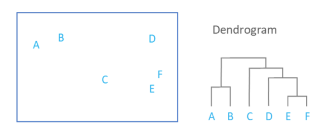
Hierarchical clustering is used to place our assets into clusters suggested by the data and not by previously defined metrics. This ensures that the assets in a specific cluster maintain similarity. The objective of this step is to build a hierarchical tree in which our assets are all clustered on different levels. Conceptually, this may be difficult for some to understand, which is why we can visualize this tree through a dendrogram.
The previous image shows the hierarchical clustering process results through a dendrogram. As the square containining our assets A-F showcases the similarity between each other, we can understand how the assets are clustered. Keep in mind that we are using agglomerative clustering, which assumes each data point to be an individual cluster at the start.
First, the assets E and F are clustered together as they are the most similar. This is followed by the clustering of assets A and B. From this point, the clustering algorithm then includes asset D (and subsequently asset C) into the first clustering pair of assets E and F. Finally, the asset pair A and B is then clustered with the rest of the assets in the last step.
So you now may be asking, how does the algorithm know which assets to cluster together? Of course, we can visually see the distance between each asset, but our algorithm cannot. There are a few widely used methods for calculating the measure of distance/similarity within our algorithm:
- Single Linkage – the distance between two clusters it the minimum distance between any two points in the clusters
- Complete Linkage – the distance between two clusters is the maximum of the distance between any two points in the clusters
- Average Linkage – the distance between two clusters is the average of the distance between any two points in the clusters
- Ward Linkage – the distance between two clusters is the increase of the squared error from when two clusters are merged
Thankfully, we can easily implement each linkage algorithm within the PortfolioLab library, allowing us to quickly compare the results to each other.
Selecting the Optimal Number of Clusters
Once our assets are all clustered in a hierarchical tree, we run into the problem of not knowing the optimal number of clusters for our weight allocations. We can use the Gap statistic for calculating our optimal number of clusters.
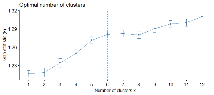
The Gap statistic is used as a measure for calculating our optimal number of clusters. It compares the total within intra-cluster variation for different values of k (with k being the number of clusters) with their expected values under null reference distribution of the data. Informally, this means that we should select the number of clusters which maximizes our Gap statistic before the rate of change begins to slow down.
For example, in the following graph, the optimal number of clusters selected would be 6.
At this stage in the algorithm, we have clustered all our assets into a hierarchical tree and selected the optimal number of clusters using the Gap statistic. We will now move onto recursive bisection.
Recursive Bisection
In this step, portfolio weights for each of the tree clusters are calculated. Based on our dendrogram structure, the recursive bisection step recursively divides our tree following an Equal Risk Contribution allocation. An Equal Risk Contribution allocation makes sure that each asset contributes equally to the portfolio’s volatility.
For example, consider a portfolio with asset allocations of 50% in stocks and 50% in bonds. While the asset allocation of this portfolio is equal with respect to our asset classes, our risk allocation is not. Depending on the nature of our stocks and bonds, our risk allocation for this portfolio can be near 90% portfolio risk in stocks and only 10% portfolio risk in bonds. By following an Equal Risk Contribution allocation method, this ensures that the recursive bisection step in our algorithm will distribute portfolio weights equally in terms of risk allocation and not in terms of asset allocation.
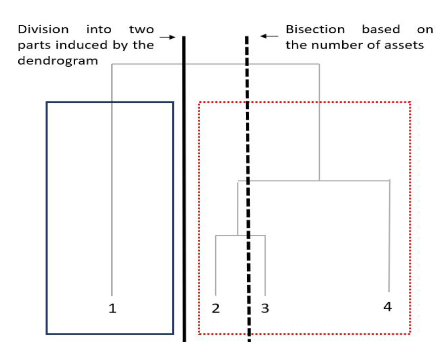
In the following image, we can see how recursive bisection splits the dendrogram by structure, and not based on assets. This is a key part of the HERC algorithm and is one of the reasons as to how HERC distinguishes itself from the HRP algorithm which breaks down the tree based on the number of assets.
Naive Risk Parity for Weight Allocations
Having calculated the cluster weights in the previous step, this step calculates the final asset weights. Within the same cluster, an initial set of weights – – is calculated using the naive risk parity allocation. In this approach, assets are allocated weights in proportion to the inverse of their respective risk; higher risk assets will receive lower portfolio weights, and lower risk assets will receive higher weights. Here the risk can be quantified in different ways – variance, CVaR, CDaR, max daily loss etc… The final weights are given by the following equation:
where, refers to naive risk parity weights of assets in the
cluster and
is the weight of the
cluster calculated in Step-3.
Using PortfolioLab’s HERC Implementation
In this section, we will go through a working example of using the HERC implementation provided by PortfolioLab and test it on a portfolio of assets.
# importing our required libraries
import pandas as pd
import numpy as np
import matplotlib.pyplot as plt
import matplotlib.patches as mpatches
from portfoliolab.clustering import HierarchicalEqualRiskContribution
Choosing the Dataset
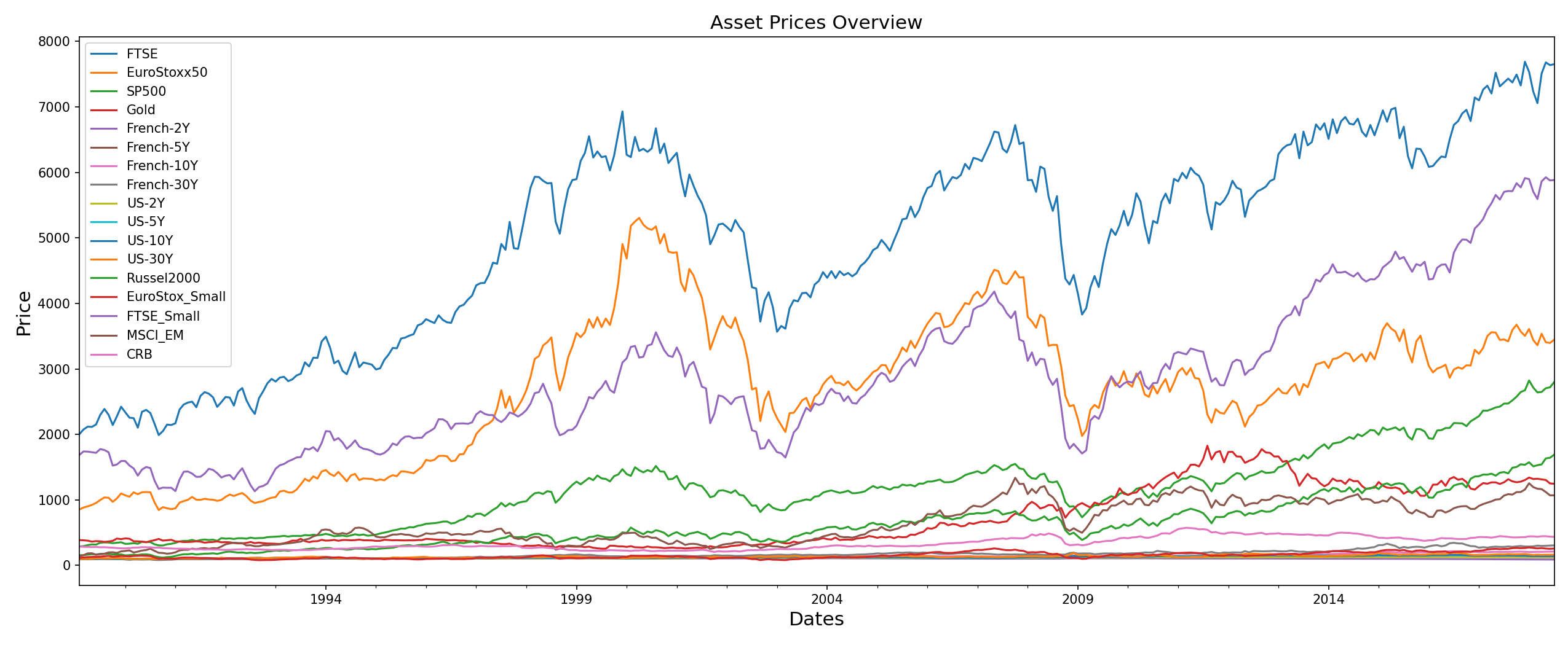
In this example, we will be working with historical closing-price data for 17 assets. The portfolio consists of diverse set of assets ranging from commodities to bonds and each asset exhibits different risk-return characteristics. You can download the dataset CSV file from our research repository here
# reading in our data
raw_prices = pd.read_csv('assetalloc.csv',
                         sep=';',
                         parse_dates=True,
                         index_col='Dates')
stock_prices = raw_prices.sort_values(by='Dates')
stock_prices.head()stock_prices.resample('M').last().plot(figsize=(17,7))
plt.ylabel('Price', size=15)
plt.xlabel('Dates', size=15)
plt.title('Asset Prices Overview', size=15)
plt.show()
The specific set of assets was chosen for two reasons:
- This is the same dataset used by Dr. Raffinot in the original HERC paper. By testing our implementation on the same data, we wanted to make sure that the results are in sync with the original results. This ensures the correctness of PortfolioLab’s implementation.
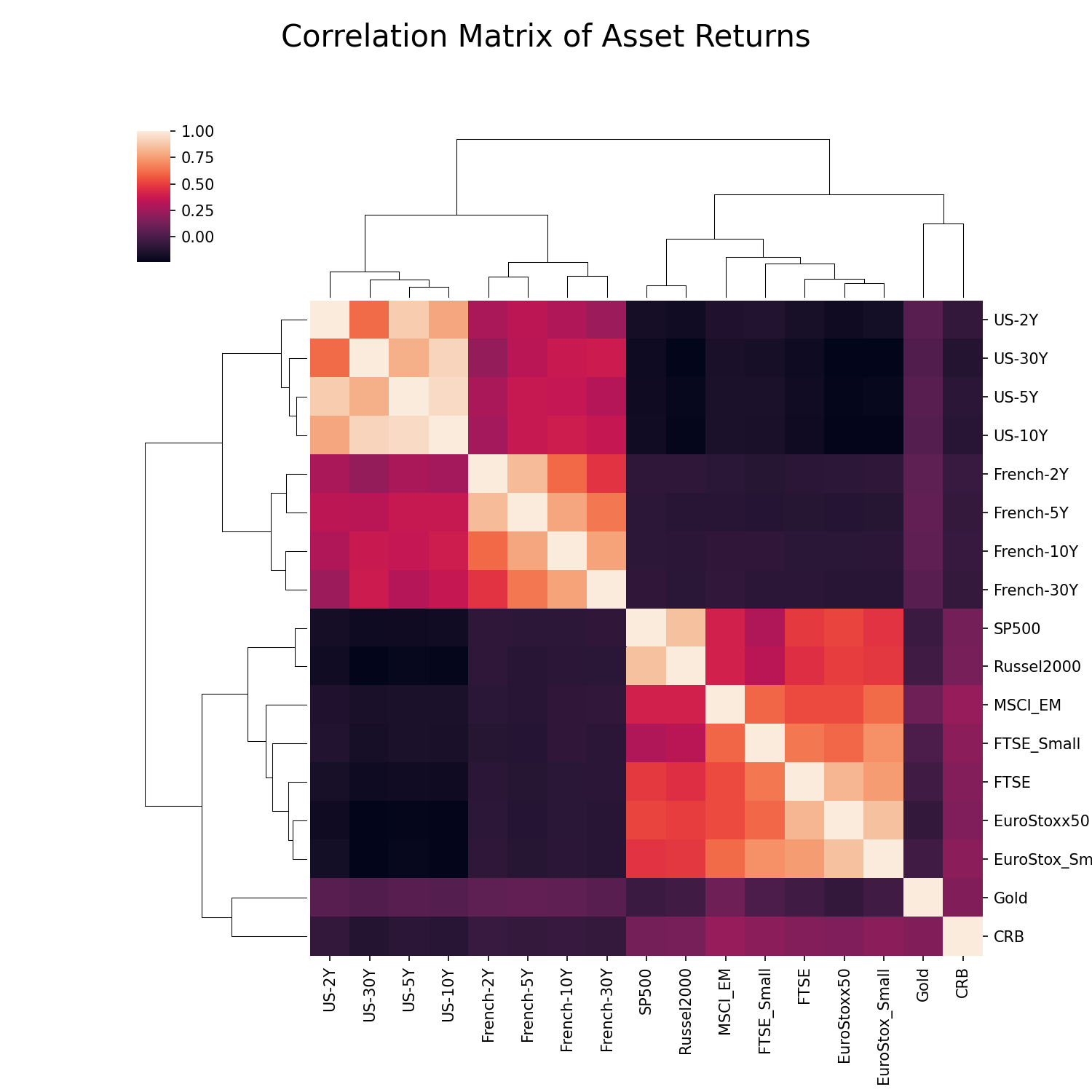
- The specific set of securities have very good clustering structure which is important for hierarchical based algorithms. If you look at the visual representation of the correlation matrix below, the inherent clusters can be clearly identified.
Calculating the Optimal Weight Allocations
Now that we have our data loaded in, we can make use of the HierarchicalEqualRiskContribution class from PortfolioLab to construct our optimized portfolio. First we must instantiate our class and then run the allocate() method to optimize our portfolio.
Keep in mind that PortfolioLab currently supports the following metrics for calculating weight allocations:
- ‘variance’: The variance of the clusters is used as a risk metric
- ‘standard_deviation’: The standard deviation of the clusters is used as a risk metric
- ‘equal_weighting’: All clusters are weighted equally with respect to the risk
- ‘expected_shortfall’: The expected shortfall of the clusters is used as a risk metric
- ‘conditional_drawdown_risk’: The conditional drawdown at risk of the clusters is used as a risk metric
PortfolioLab also supports all four linkage algorithms discussed in this post, though the default method is set as the Ward Linkage algorithm.
The allocate() method for the HierarchicalEqualRiskContribution object requires three parameters to run:
- asset_names (a list of strings containing the asset names)
- asset_prices (a dataframe of historical asset prices – daily close)
- risk_measure (the type of risk representation to use – PortfolioLab currently supports 5 different solutions)
Note: The list of asset names is not a necessary parameter. If your input data is in the form of a dataframe, it will use the column names as the default asset names.
Users can also specify:
- The type of linkage algorithm (shown below)
- The confidence level used for calculating expected shortfall and conditional drawdown at risk
- The optimal number of clusters for clustering
For simplicity, we will only be working with the three required parameters and also specifying our linkage algorithm of choice. In the example shown below, we are using an equal_weighting solution and the Ward Linkage algorithm.
herc = HierarchicalEqualRiskContribution()
herc.allocate(asset_names=stock_prices.columns,
              asset_prices=stock_prices,
              risk_measure="equal_weighting",
              linkage="ward")

# plotting our optimal portfolio
herc_weights = herc.weights
y_pos = np.arange(len(herc_weights.columns))

plt.figure(figsize=(25,7))
plt.bar(list(herc_weights.columns), herc_weights.values[0])
plt.xticks(y_pos, rotation=45, size=10)
plt.xlabel('Assets', size=20)
plt.ylabel('Asset Weights', size=20)
plt.title('HERC Portfolio Weights', size=20)
plt.show()
We can observe from the above plot that many assets have been assigned equal weights. However, there is still a visible difference in the allocations. Let us see the reason behind this by visualising the tree structure.
Plotting the Clusters
The clusters can be visualised by calling the plot_clusters() method. This will plot the dendrogram tree which is the standard way of visualising hierarchical clusters.
plt.figure(figsize=(17,7))
herc.plot_clusters(assets=stock_prices.columns)
plt.title('HERC Dendrogram', size=18)
plt.xticks(rotation=45)
plt.show()
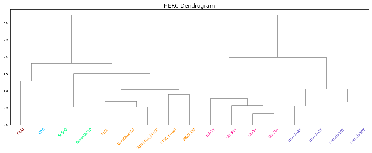
In this graph, the different colors in the x-labels represent the clusters that the stocks belong to. Through visual analysis, we can count that the optimal number of clusters determined by the Gap statistic is 6 for our dataset. We can also confirm this by printing out our optimal number of clusters through the ‘optimal_num_clusters’ attribute.
print("Optimal Number of Clusters: " + str(herc.optimal_num_clusters))
This shows why some assets received similar weights. At each point of bisection, the left and right clusters are assigned equal weights. This results in both the US and French clusters getting the same weight allocation which is then distributed equally among all assets. Hence, all the US and French assets have the same weight allocations.
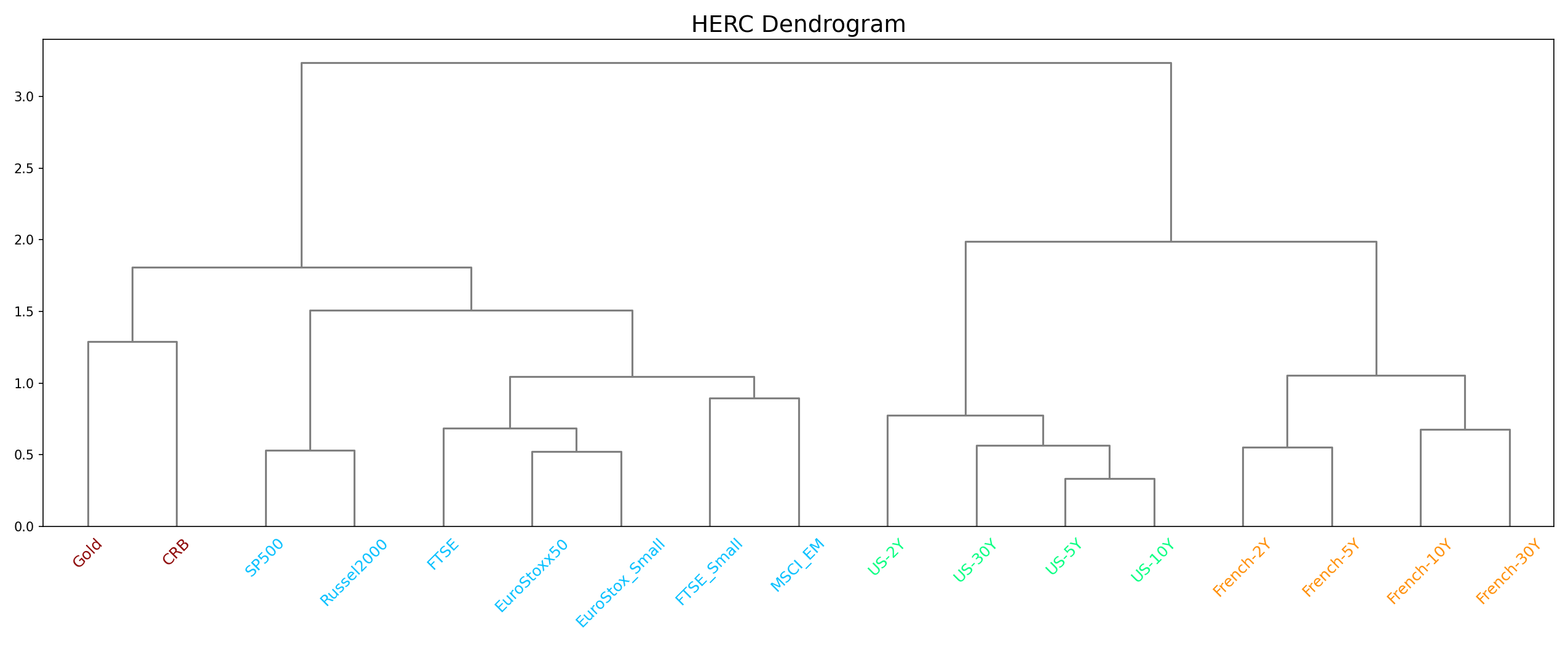
Changing the optimal number of clusters can lead to very different weight allocations. You can play around with this number by passing different values through the optimal_num_clusters parameter and understanding how the weights change. For example, in the following code snippet, we look at the clusters identified by the algorithm when the optimal number of clusters is 4.
herc = HierarchicalEqualRiskContribution()
herc.allocate(asset_prices=stock_prices,
              optimal_num_clusters=4,
              risk_measure="equal_weighting")

# Plot clusters
plt.figure(figsize=(17,7))
herc.plot_clusters(assets=stock_prices.columns)
plt.title('HERC Dendrogram', size=18)
plt.xticks(rotation=45)
plt.show()

# Plotting optimal portfolio
herc_weights = herc.weights
y_pos = np.arange(len(herc_weights.columns))

plt.figure(figsize=(25,7))
plt.bar(list(herc_weights.columns), herc_weights.values[0])
plt.xticks(y_pos, rotation=45, size=10)
plt.xlabel('Assets', size=20)
plt.ylabel('Asset Weights', size=20)
plt.title('HERC Portfolio Weights', size=20)
plt.show()
You can observe that Gold and CRB have now been grouped into one cluster. Similarly, SP500 and Russel2000 are now in the same cluster as the other assets like FTSE and MSCI. Due to this, the weight allocations have also changed slightly, as can be observed in the following figure.
Using Custom Input with PortfolioLab
PortfolioLab also provides users with a lot of customizability when it comes to creating their optimal portfolios. Instead of providing the raw historical closing prices for the assets, users can input the asset returns, a covariance matrix of asset returns, and expected asset returns to calculate their optimal portfolio.
The following parameters in the allocate() method are utilized in order to construct a custom use case:
- ‘asset_returns’: (pd.DataFrame/NumPy matrix) A matrix of asset returns
- ‘covariance_matrix’: (pd.DataFrame/NumPy matrix) A covariance matrix of asset returns
In this example, we will be constructing the same optimized portfolio as the first example, utilizing an equal_weighting solution with the Ward Linkage algorithm. As we already know the optimal number of clusters, we will also be passing that in as a parameter to save on computation time.
To make some of the necessary calculations, we will make use of the ReturnsEstimators class provided by PortfolioLab.
# importing ReturnsEstimation class from PortfolioLab
from portfoliolab.estimators import ReturnsEstimators

# calculating our asset returns
returns = ReturnsEstimators.calculate_returns(stock_prices)

# calculating our covariance matrix
cov = returns.cov()

# from here, we can now create our portfolio
herc_custom = HierarchicalEqualRiskContribution()
herc_custom.allocate(asset_returns=returns,
                     covariance_matrix=cov,
                     risk_measure='equal_weighting',
                     linkage='ward',
                     optimal_num_clusters=6)
You can observe that these are exactly the same portfolio we got when passing raw asset prices. You can further play around with the different risk measures mentioned previously and generate different types of portfolios.
Conclusion and Further Reading
Through this post, we learned the intuition behind Thomas Raffinot’s Hierarchical Equal Risk Contribution portfolio optimization algorithm and also saw how we can utilize PortfolioLab’s implementation to apply this technique out-of-the-box. HERC is a powerful algorithm that can produce robust portfolios which avoids many of the problems seen with Modern Portfolio Theory and Hierarchical Risk Parity.
The following links provide a more detailed exploration of the algorithms for further reading.
Official PortfolioLab Documentation:
Research Papers:
- Hierarchical Equal Risk Contribution – Original Paper
- Hierarchical Clustering Based Asset Allocation – Original Paper

