Online Portfolio Selection: Mean Reversion
By Alex Kwon
Join the Reading Group and Community: Stay up to date with the latest developments in Financial Machine Learning!
Mean Reversion is an effective quantitative strategy based on the theory that prices will revert back to its historical mean. A basic example of mean reversion follows the benchmark of Constant Rebalanced Portfolio. By setting a predetermined allocation of weight to each asset, the portfolio shifts its weights from increasing to decreasing ones. This module will implement four types of mean reversion strategies:
- Passive Aggressive Mean Reversion
- Confidence Weighted Mean Reversion
- Online Moving Average Reversion
- Robust Median Reversion.
Through this blog post, the importance of hyperparameters is highlighted, as the choices greatly affect the outcome of returns. Many of the hyperparameters for traditional research has been chosen by looking at the data in hindsight, and fundamental analysis of each dataset and market structure is required to profitably implement this strategy in a real-time market scenario.
We will be introducing the applications of these popular strategies with the ease of using PortfolioLab’s newest module. I hope that the newfound interests from these topics will spur more development as well as assist the research process for many others in the field.
Passive Aggressive Mean Reversion
Passive Aggressive Mean Reversion alternates between a passive and aggressive approach to the current market conditions. The strategy can effectively prevent a huge loss and maximize returns by setting a threshold for mean reversion.
PAMR takes in a variable ![]() , a threshold for the market condition. If the portfolio returns for the period are below
, a threshold for the market condition. If the portfolio returns for the period are below ![]() , then PAMR will passively keep the previous portfolio, whereas if the returns are above the threshold, the portfolio will actively rebalance to the less performing assets.
, then PAMR will passively keep the previous portfolio, whereas if the returns are above the threshold, the portfolio will actively rebalance to the less performing assets.
In a way, ![]() can be interpreted as the maximum loss for the portfolio. It is most likely that the asset that decreased in prices for the period will bounce back, but there are cases where some companies plummet in value. PAMR is an effective algorithm that will prevent huge losses in blindly following these assets. Three different methods of PAMR have been implemented in the module with different levels of aggressiveness towards mean reversion.
can be interpreted as the maximum loss for the portfolio. It is most likely that the asset that decreased in prices for the period will bounce back, but there are cases where some companies plummet in value. PAMR is an effective algorithm that will prevent huge losses in blindly following these assets. Three different methods of PAMR have been implemented in the module with different levels of aggressiveness towards mean reversion.
Confidence Weighted Mean Reversion
Extending from PAMR, Confidence Weighted Mean Reversion looks at the autocovariance across all assets. Instead of focusing on a single asset’s deviation from the original price, CWMR takes in second-order information about the portfolio vector as well to formulate a set of weights.
For CWMR, we introduce ![]() , a measure of anti-confidence in the portfolio weights, where a smaller value represents higher confidence for the corresponding portfolio weights.
, a measure of anti-confidence in the portfolio weights, where a smaller value represents higher confidence for the corresponding portfolio weights.
The problem can be interpreted as maximizing the portfolio confidence by minimizing ![]() given a confidence interval
given a confidence interval ![]() determined by the threshold,
determined by the threshold, ![]() . Two different solutions to the problem were implemented in the module with the standard deviation and variance method.
. Two different solutions to the problem were implemented in the module with the standard deviation and variance method.
Online Moving Average Reversion
Traditional mean reversion techniques have an underlying assumption that the next price relative is inversely proportional to the latest price relative; however, mean reversion trends are not limited to a single period. Unlike traditional reversion methods that rely on windows of just one, OLMAR looks to revert to the moving average of price data.
OLMAR proposes two different moving average methods: Simple Moving Average and Exponential Moving Average. From these moving average methods, the strategy predicts the next period’s price relative, and the strategy iteratively updates its new weights.
Robust Median Reversion
Robust Median Reversion extends the previous Online Moving Average Reversion by introducing the L1 median of the specified windows. Instead of reverting to a moving average, RMR reverts to the L1 median estimator, which proves to be a more effective method of predicting the next period’s price because financial data is inherently noisy and contains many outliers.
Calculating the L1 median is computationally inefficient, so the Modified Weiszfeld Algorithm is used to speed up the process.
Data
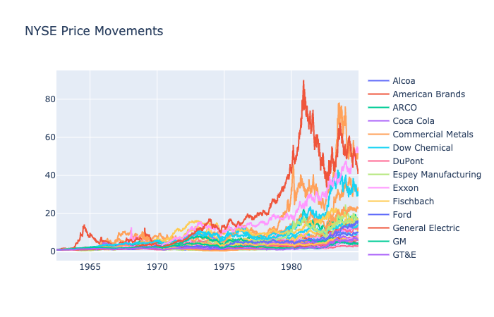
We will be using 6 different datasets, and if you would like to learn more about each dataset, exploratory analysis is available here.
- 36 NYSE Stocks from 1962 to 1984 by Cover
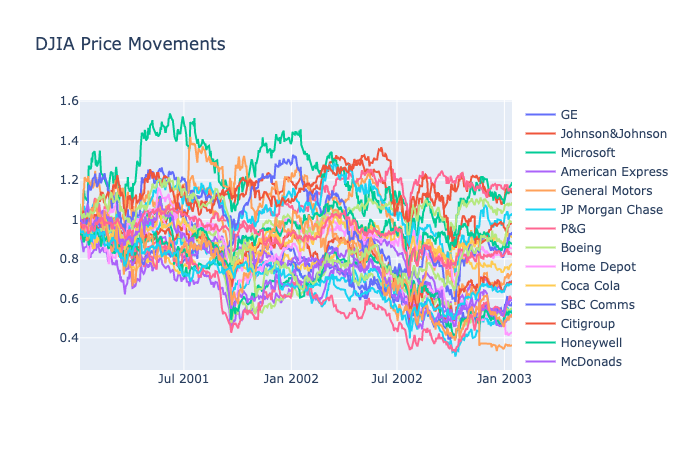
- 30 DJIA Stocks from 2001 to 2003 by Borodin
- 88 TSE Stocks from 1994 to 1998 by Borodin
- 25 Largest S&P500 Stocks from 1998 to 2003 by Borodin
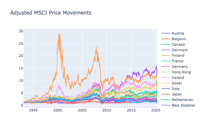
- 23 MSCI Developed Market Indices from 1993 to 2020 by Alex Kwon
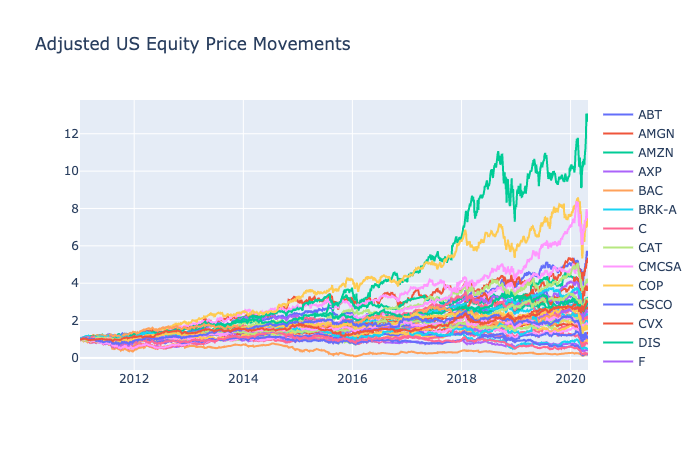
- 44 Largest US Stocks from 2011 to 2020 by Alex Kwon
We will be using Optuna to examine the effects of parameters.
NYSE: 1962-1984
PAMR results on NYSE indicate the dependency on epsilon value over agg(aggressiveness). A low value of epsilon, one that is close to 0, is ideal in this strategy and indicates the preference for passive mean reversion.
CWMR results vary over the intervals of confidence and epsilon. The majority of the trials returned around the same magnitude; however, for certain parameters, CWMR produced extremely high returns. The high returns have a common parameter of a high epsilon value of 1.
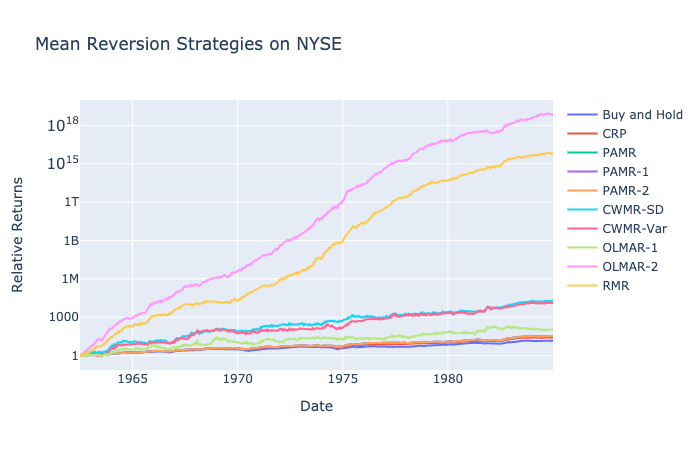
OLMAR’s returns are exponentially higher than other mean reversion techniques so far with magnitudes of ![]() . OLMAR returns are more dependent on the alpha and window parameters that choose the moving averages rather than epsilon. Interestingly, a window of 23 was ideal for OLMAR-1, and an alpha of 0.35 was ideal for OLMAR-2. A tendency of mean reversion for a longer period appears for the NYSE dataset proven by the relatively lower value of alpha and window of closer to three weeks.
. OLMAR returns are more dependent on the alpha and window parameters that choose the moving averages rather than epsilon. Interestingly, a window of 23 was ideal for OLMAR-1, and an alpha of 0.35 was ideal for OLMAR-2. A tendency of mean reversion for a longer period appears for the NYSE dataset proven by the relatively lower value of alpha and window of closer to three weeks.
From the graph, we can notice that darker lines indicate higher returns. The majority of the dark line goes through a high epsilon and low window value. The range for the number of iterations and epsilon is wide, but the results were primarily dependent on the window value of 2.
OLMAR-2 and RMR returns are significantly higher than any other strategies with astronomical returns of ![]() .
.
DJIA: 2001-2003
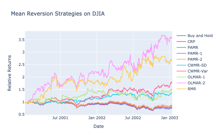
Similarly to NYSE, DJIA data is dependent on the epsilon parameter. A lower value of epsilon, closer to 0, produced higher returns regardless of aggressiveness.
CWMR produces a similar graph to NYSE’s. Epsilon of 1 continues to be the ideal parameter; however, confidence is different for CWMR-Var and CWMR-SD. The best confidence value for the variance method is 1, whereas the standard deviation’s parameter is closer to 0.
OLMAR parameters suggest a similar trend where the epsilon parameter does not significantly affect results. A window of 8 represents a shorter mean reversion trend with the DJIA dataset, and a low alpha value of 0.1 indicates less importance on the current weights as a parameter for price prediction.
Higher returns were achieved from high epsilon, a lower number of iterations, and a window range of 12 to 16. This is in contrast to the window range suggested by OLMAR-1, where 8 had the highest returns. A higher window value for RMR compared to OLMAR-1 indicate that the noise in price data is more effectively reduced with a wider range of window.
Mean reversion strategies perform significantly better than other benchmarks. For a period of a continuous downtrend, OLMAR-2 and RMR each have triple and double returns when most other strategies are stagnant around 1. Mean reversion provides promising returns for a long bear market.
TSE: 1994-1998
TSE suggests a different ideal epsilon value from the two previous datasets. Instead of 0, the best epsilon value is 0.6. The strategy performed an aggressive strategy for portfolio returns that were above 0.6 and performed a passive strategy for periods with returns less than 0.6. The returns are also relatively less sensitive to epsilon value as models with epsilon value between 0.4 and 1 have similar returns.
CWMR parameters are very different from the previous datasets. For the standard deviation method, epsilon values have minimal effect on returns as the highest drive was the low value of confidence around 0.1. For the variance method, a confidence value of 0.5 displayed significantly higher returns with epsilon not having as much effect as it did on the standard deviation method.
TSE also represents a longer mean reversion window of 23 and an alpha of 0.9. The difference between the two parameters is noteworthy as a high value of alpha indicates a stronger weighting for recent prices; however, the high window value of 23 suggests that the periods are reliant on a more longer-term.
RMR results indicate that the most important parameter is the number of windows. A window of 2 had the highest returns regardless of epsilon and number of iterations. This is in line with the OLMAR-2 strategy that had the best returns with a high alpha value. A shorter window frame was a better indicator of future prices for the TSE dataset.
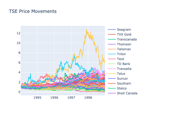
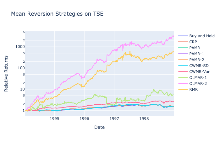
OLMAR-2 and RMR continue to lead in returns with OLMAR-1 being a distant third. Shorter mean reversion trends proved to be a successful strategy for TSE.
SP500: 1998-2003
Epsilon of 0 proved to have the highest return as aggressiveness continues to have minimal impact on our returns.
CWMR-Var had its highest and lowest returns at a confidence value of 0.45. CWMR continues to be sensitive to its hyperparameters as even the slightest deviations of parameters return vastly different returns for its models.
For SP500, a window of 2 and an alpha of 0.4 produced the highest returns. OLMAR-1 returns vary for most parameter choices and do not indicate a strong trend in any direction; however, OLMAR-2 has a clear alpha value that maximizes returns and is more robust to different parameter choices in the range between 0.3 and 0.5.
The darkest lines for RMR pass through high epsilon, a low number of iterations, and a window range between 4 and 8.
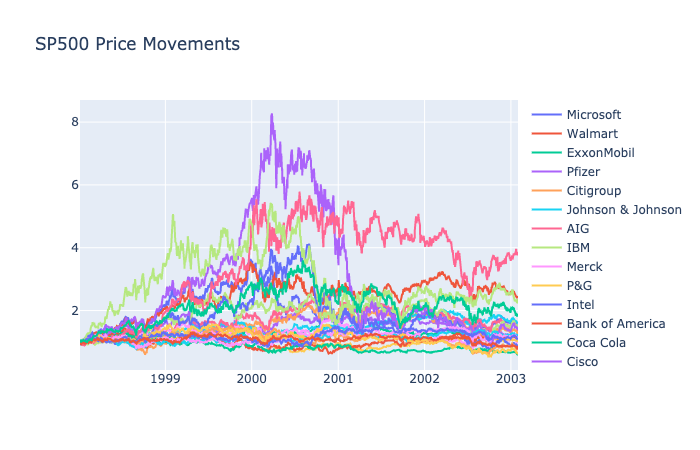
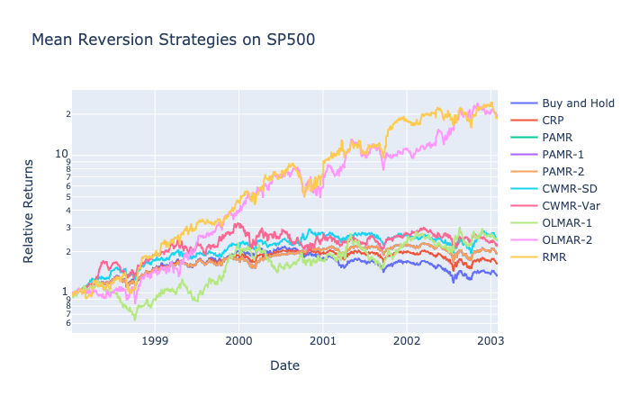
OLMAR-2 and RMR produce the highest returns as the rest of the strategies fail to increase by more than 2 times the original value.
MSCI: 1993-2020
Aggressive mean reversion was less preferred for MSCI with a low epsilon value preferred.
For both sets, epsilon of 1 had the highest returns with low confidence for CWMR-SD and high confidence for CWMR-Var. CWMR continues to provide models that are extremely sensitive to hyperparameter choices.
A window of 8 was optimal for mean reversion prediction for OLMAR-1, and OLMAR-2 had an optimal alpha value close to 0.1.
RMR values were highest for high epsilon, a low number of iteration, and a window range of 12 to 15. The relatively higher optimal window value is similar to the optimal parameter for OLMAR-2. Both indicate a longer mean reversion expectancy regarding price predictions.
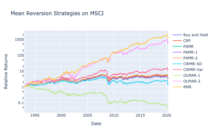
Not too surprisingly, OLMAR-2 and RMR produce the highest returns by more than 100 times in returns compared to other strategies. OLMAR-1, which typically represented a robust model, actually failed to have positive returns and approached a portfolio value closer to 0.
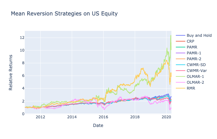
US Equity: 2011-2020
Unlike the majority of the previous datasets, higher epsilon was preferred as there were more daily mean reversion trends with US equity data.
A confidence of 0.45 for both models produced the highest returns; however, the lack of clean pattern and direction for the parameters represent the difficulty of applying CWMR to real live trading environments.
A window of 11 and alpha of 0.1 proved to have the highest returns. The simple moving average trend was closer to a week-long, and for the first time, OLMAR-2 actually has negative returns compared to its original portfolio value.
The range of dark lines over the entire range for epsilon and number of iterations indicate that the most important parameter is the number of windows. RMR had the highest returns for windows in range of 18 to 23. This is a higher value compared to OLMAR-1’s window of 8 and is an example where a longer window range was more important as a variable to predict future prices due to the noise in daily price data.
OLMAR-1 and RMR were the best performing strategies with OLMAR-2 lagging much behind its peers.
Conclusion
Mean reversion can be formulated in multiple methods. From a simple constant rebalanced portfolio to a complex robust median reversion, the strategy can employ endless techniques to find the most profitable set of portfolio weights. The blog post covered a wide range of mean reversion strategies employed in PortfolioLab’s newest Online Portfolio Selection module, and readers will be able to replicate results using the simple methods of the new module.
The next notebook will focus on Pattern Matching.
If you enjoyed reading this please remember to leave us a star on GitHub and become a sponsor on Patreon to have exclusive access to our Slack channel!
Additional Reading:
Reference
- Li, B. and Hoi, S.C.H., 2018. Online portfolio selection: principles and algorithms. Crc Press.
- Li, B., Zhao, P., Hoi, S.C. and Gopalkrishnan, V., 2012. PAMR: Passive aggressive mean reversion strategy for portfolio selection. Machine learning, 87(2), pp.221-258.
- Li, B., Hoi, S.C., Zhao, P. and Gopalkrishnan, V., 2013. Confidence weighted mean reversion strategy for online portfolio selection. ACM Transactions on Knowledge Discovery from Data (TKDD), 7(1), pp.1-38.
- Li, B. and Hoi, S.C., 2012. On-line portfolio selection with moving average reversion. arXiv preprint arXiv:1206.4626.
- Huang, D., Zhou, J., Li, B., Hoi, S.C. and Zhou, S., 2016. Robust median reversion strategy for online portfolio selection. IEEE Transactions on Knowledge and Data Engineering, 28(9), pp.2480-2493.

![DJIA RMR Epsilon [1, 25] N_iter [2, 1000] Window [2, 30]](https://hudsonthames.org/wp-content/uploads/2020/05/newplot-18-2.png)
![PAMR Epsilon [0, 1.5]](https://hudsonthames.org/wp-content/uploads/2020/05/newplot-43.png)
![PAMR-1 Epsilon [0, 1.5] Aggressiveness [1e-3, 1e5]](https://hudsonthames.org/wp-content/uploads/2020/05/newplot-1-3.png)
![PAMR-2 Epsilon [0, 1.5] Aggressiveness [1e-3, 1e5]](https://hudsonthames.org/wp-content/uploads/2020/05/newplot-2-3.png)
![NYSE CWMR-Var Epsilon [0, 1] Confidence [0, 1]](https://hudsonthames.org/wp-content/uploads/2020/05/newplot-4-3.png)
![NYSE CWMR-SD Epsilon [0, 1] Confidence [0, 1]](https://hudsonthames.org/wp-content/uploads/2020/05/newplot-3-3.png)
![NYSE OLMAR-1 Epsilon [2, 25] Window [2, 30]](https://hudsonthames.org/wp-content/uploads/2020/05/newplot-5-3.png)
![NYSE OLMAR-2 Epsilon [2, 25] Alpha [0, 1]](https://hudsonthames.org/wp-content/uploads/2020/05/newplot-6-3.png)
![NYSE RMR Epsilon [1, 25] N_iter [2, 1000] Window [2, 30]](https://hudsonthames.org/wp-content/uploads/2020/05/newplot-8-3.png)
![DJIA PAMR Epsilon [0, 1.5]](https://hudsonthames.org/wp-content/uploads/2020/05/newplot-10-2-495x400.png)
![DJIA PAMR-1 Epsilon [0, 1.5] Aggressiveness [1e-3, 1e5]](https://hudsonthames.org/wp-content/uploads/2020/05/newplot-11-2-495x400.png)
![DJIA PAMR-2 Epsilon [0, 1.5] Aggressiveness [1e-3, 1e5]](https://hudsonthames.org/wp-content/uploads/2020/05/newplot-12-2-495x400.png)
![DJIA CWMR-Var Epsilon [0, 1] Confidence [0, 1]](https://hudsonthames.org/wp-content/uploads/2020/05/newplot-14-2.png)
![DJIA CWMR-SD Epsilon [0, 1] Confidence [0, 1]](https://hudsonthames.org/wp-content/uploads/2020/05/newplot-13-2.png)
![DJIA OLMAR-1 Epsilon [2, 25] Window [2, 30]](https://hudsonthames.org/wp-content/uploads/2020/05/newplot-15-2.png)
![DJIA OLMAR-2 Epsilon [2, 25] Alpha [0, 1]](https://hudsonthames.org/wp-content/uploads/2020/05/newplot-16-3.png)
![TSE PAMR Epsilon [0, 1.5]](https://hudsonthames.org/wp-content/uploads/2020/05/newplot-20-2.png)
![TSE PAMR-1 Epsilon [0, 1.5] Aggressiveness [1e-3, 1e5]](https://hudsonthames.org/wp-content/uploads/2020/05/newplot-21-2.png)
![TSE PAMR-2 Epsilon [0, 1.5] Aggressiveness [1e-3, 1e5]](https://hudsonthames.org/wp-content/uploads/2020/05/newplot-22-2.png)
![TSE CWMR-Var Epsilon [0, 1] Confidence [0, 1]](https://hudsonthames.org/wp-content/uploads/2020/05/newplot-24-2.png)
![TSE CWMR-SD Epsilon [0, 1] Confidence [0, 1]](https://hudsonthames.org/wp-content/uploads/2020/05/newplot-23-2.png)
![TSE OLMAR-1 Epsilon [2, 25] Window [2, 30]](https://hudsonthames.org/wp-content/uploads/2020/05/newplot-25-2.png)
![TSE OLMAR-2 Epsilon [2, 25] Alpha [0, 1]](https://hudsonthames.org/wp-content/uploads/2020/05/newplot-26-3.png)
![TSE RMR Epsilon [1, 25] N_iter [2, 1000] Window [2, 30]](https://hudsonthames.org/wp-content/uploads/2020/05/newplot-27-3.png)
![SP500 PAMR Epsilon [0, 1.5]](https://hudsonthames.org/wp-content/uploads/2020/05/newplot-29-1.png)
![SP500 PAMR-1 Epsilon [0, 1.5] Aggressiveness [1e-3, 1e5]](https://hudsonthames.org/wp-content/uploads/2020/05/newplot-30-1.png)
![SP500 PAMR-2 Epsilon [0, 1.5] Aggressiveness [1e-3, 1e5]](https://hudsonthames.org/wp-content/uploads/2020/05/newplot-31-1.png)
![SP500 CWMR-Var Epsilon [0, 1] Confidence [0, 1]](https://hudsonthames.org/wp-content/uploads/2020/05/newplot-32-1.png)
![SP500 CWMR-SD Epsilon [0, 1] Confidence [0, 1]](https://hudsonthames.org/wp-content/uploads/2020/05/newplot-33-1.png)
![SP500 OLMAR-1 Epsilon [2, 25] Window [2, 30]](https://hudsonthames.org/wp-content/uploads/2020/05/newplot-38-1.png)
![SP500 OLMAR-2 Epsilon [2, 25] Alpha [0, 1]](https://hudsonthames.org/wp-content/uploads/2020/05/newplot-39-1.png)
![SP500 RMR Epsilon [1, 25] N_iter [2, 1000] Window [2, 30]](https://hudsonthames.org/wp-content/uploads/2020/05/newplot-40-1.png)
![MSCI PAMR Epsilon [0, 1.5]](https://hudsonthames.org/wp-content/uploads/2020/05/newplot-42-1.png)
![MSCI PAMR-1 Epsilon [0, 1.5] Aggressiveness [1e-3, 1e5]](https://hudsonthames.org/wp-content/uploads/2020/05/newplot-43-1.png)
![MSCI PAMR-2 Epsilon [0, 1.5] Aggressiveness [1e-3, 1e5]](https://hudsonthames.org/wp-content/uploads/2020/05/newplot-44.png)
![MSCI CWMR-Var Epsilon [0, 1] Confidence [0, 1]](https://hudsonthames.org/wp-content/uploads/2020/05/newplot-45.png)
![MSCI CWMR-SD Epsilon [0, 1] Confidence [0, 1]](https://hudsonthames.org/wp-content/uploads/2020/05/newplot-46.png)
![MSCI OLMAR-1 Epsilon [2, 25] Window [2, 30]](https://hudsonthames.org/wp-content/uploads/2020/05/newplot-47.png)
![MSCI OLMAR-2 Epsilon [2, 25] Alpha [0, 1]](https://hudsonthames.org/wp-content/uploads/2020/05/newplot-48.png)
![MSCI RMR Epsilon [1, 25] N_iter [2, 1000] Window [2, 30]](https://hudsonthames.org/wp-content/uploads/2020/05/newplot-49.png)
![US Equity PAMR Epsilon [0, 1.5]](https://hudsonthames.org/wp-content/uploads/2020/05/newplot-51.png)
![US Equity PAMR-1 Epsilon [0, 1.5] Aggressiveness [1e-3, 1e5]](https://hudsonthames.org/wp-content/uploads/2020/05/newplot-52.png)
![US Equity PAMR-2 Epsilon [0, 1.5] Aggressiveness [1e-3, 1e5]](https://hudsonthames.org/wp-content/uploads/2020/05/newplot-53.png)
![US Equity CWMR-Var Epsilon [0, 1] Confidence [0, 1]](https://hudsonthames.org/wp-content/uploads/2020/05/newplot-54.png)
![US Equity CWMR-SD Epsilon [0, 1] Confidence [0, 1]](https://hudsonthames.org/wp-content/uploads/2020/05/newplot-55.png)
![US Equity OLMAR-1 Epsilon [2, 25] Window [2, 30]](https://hudsonthames.org/wp-content/uploads/2020/05/newplot-56.png)
![US Equity OLMAR-2 Epsilon [2, 25] Alpha [0, 1]](https://hudsonthames.org/wp-content/uploads/2020/05/newplot-57.png)
![US Equity RMR Epsilon [1, 25] N_iter [2, 1000] Window [2, 30]](https://hudsonthames.org/wp-content/uploads/2020/05/newplot-58.png)
