Online Portfolio Selection: Momentum
By Alex Kwon
Join the Reading Group and Community: Stay up to date with the latest developments in Financial Machine Learning!
Today we will be exploring the second chapter of our newest online portfolio selection module, momentum.
Momentum strategies have been a popular quantitative strategy in recent decades as the simple but powerful trend-following allows investors to exponentially increase their returns. This module will implement two types of momentum strategies with one following the best-performing assets in the last period and the other following the Best Constant Rebalanced Portfolio until the last period.
Before we dive into momentum, I would like to first thank everyone for all the comments and feedback that I received from the previous blog post. It has been incredibly motivating and rewarding to receive many compliments as well as constructive critiques.
The focus of this post will be on introducing the applications of these popular strategies with the ease of using PortfolioLab’s newest module. I hope that the newfound interests from these topics will spur more development as well as assist the research process for many others in the field.
Exponential Gradient
Exponential Gradient strategies track the best performing stock with a learning rate, ![]() , but also regularizes the new portfolio weight to prevent drastic changes from the previous portfolio.
, but also regularizes the new portfolio weight to prevent drastic changes from the previous portfolio.
![]()
As a review, ![]() is the portfolio weights, and
is the portfolio weights, and ![]() is the price relatives for time
is the price relatives for time ![]() .
.
Exponential Gradients have an extremely efficient computational time that scales with the number of assets, and broadly speaking, there are three update methods to iteratively update the selection of portfolio weights.
Multiplicative Update
David Helmbold first proposed a regularization term that adopts relative entropy.
![]()
Using log’s first order taylor expansion of ![]()
![]()
Multiplicative update algorithm can be stated as the following.
![]()
Gradient Projection
Instead of relative entropy, gradient projection adopts an L2-regularization term.
![]()
Gradient projection can then be iteratively updated with the following equation.
![]()
Expectation Maximization
Lastly, expectation maximization uses ![]() regularization.
regularization.
![]()
Then the corresponding update rule becomes
![]()
Follow the Leader
The biggest drawback of using Exponential Gradient is the failure to look at the changes before the latest period. Follow the Leader mediates this shortfall by directly tracking the Best Constant Rebalanced Portfolio; therefore, FTL looks at the whole history of the data and calculates the portfolio weights that would have had the maximum returns.
![]()
Follow the Regularized Leader
Follow the Regularized Leader adds an additional regularization term to prevent rapid changes each period.
![]() acts similarly to Exponential Gradient’s
acts similarly to Exponential Gradient’s ![]() .
.
![]()
Data
We will be using 6 different datasets, and if you would like to learn more about each dataset, exploratory analysis is available here.
- 36 NYSE Stocks from 1962 to 1984 by Cover
- 30 DJIA Stocks from 2001 to 2003 by Borodin
- 88 TSE Stocks from 1994 to 1998 by Borodin
- 25 Largest S&P500 Stocks from 1998 to 2003 by Borodin
- 23 MSCI Developed Market Indices from 1993 to 2020 by Alex Kwon
- 44 Largest US Stocks by from 2011 to 2020 by Alex Kwon
NYSE: 1961-1984
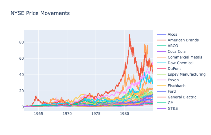
Generally, most assets in this dataset increased by a significant amount. The notable outperforming companies are American Brands and Commercial Metals, and the least performing stock, DuPont, still ended with 2.9 times returns as no stocks in this list decreased in value.
We will be using Optuna and dividing the parameters into two sets. The first set will include parameter values between 0 and 1 to emphasize the importance of adhering to the previous portfolio weights, and the second set will examine values between 1 and 100, which will present significant returns if changing weights benefit the overall returns.
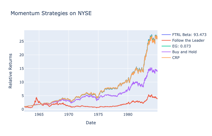
From Helmbold’s original paper, ![]() of 0.05 was suggested for Exponential Gradient, and through our tuning, we discovered that the best parameter was 0.0736, which is very similar to the suggested
of 0.05 was suggested for Exponential Gradient, and through our tuning, we discovered that the best parameter was 0.0736, which is very similar to the suggested ![]() value.
value.
Follow the Regularized Leader’s ![]() with the highest returns indicate similar returns to the highest returns by Exponential Gradient.
with the highest returns indicate similar returns to the highest returns by Exponential Gradient.
A simple buy and hold returned 12, whereas the best performing Exponential Gradient returned 26.7.
For a dataset where all stocks increase in value and a uniform buy and hold strategy is profitable, a low EG value was adequate. Huge deviations from the original portfolio weight were not necessary and blindly following the best performing asset often decreased the returns as the momentum for these sets of stocks did not continue on a daily basis.
DJIA: 2001-2003
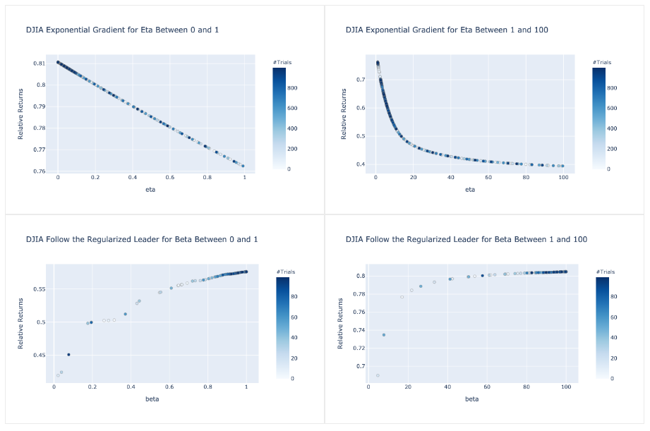
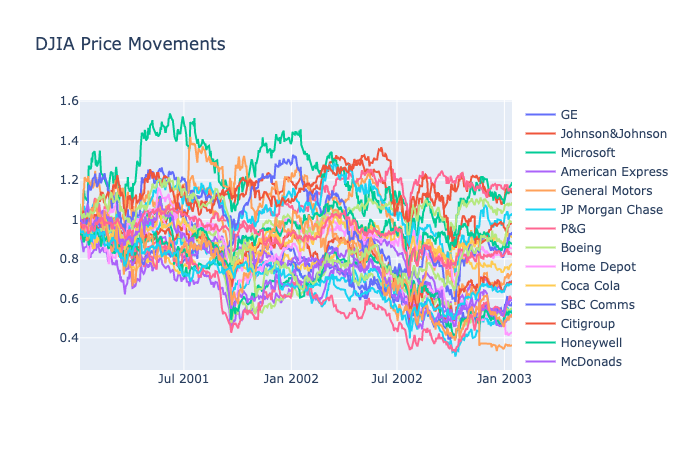
DJIA from 2001 to 2003 provides strikingly different patterns compared to the previous NYSE data. Only 5 companies increased in price as most declined at a steady rate.
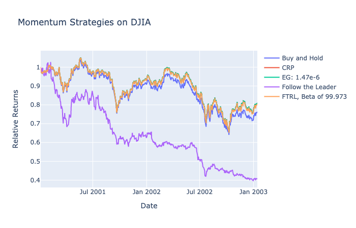
The ideal ![]() for Exponential Gradient was a value close to 0, and ideal
for Exponential Gradient was a value close to 0, and ideal ![]() was close to 100. These parameters suggest that the weights should not change from its original set value. The regularization term in FTRL prevents the strategy from tracking the BCRP, and the learning rate in EG prevents the strategy from following the Best Stock.
was close to 100. These parameters suggest that the weights should not change from its original set value. The regularization term in FTRL prevents the strategy from tracking the BCRP, and the learning rate in EG prevents the strategy from following the Best Stock.
For a market with a general downtrend, momentum strategies fail to make a significant effect on our returns. This is in line with the underlying concept for momentum where a strong trend in a direction is necessary to reap the rewards. With our current problem formulation that prevents shorting assets, a momentum strategy cannot produce meaningful returns in this environment. It is not surprising that both Exponential Gradient and Follow the Leader fail to have higher returns than a simple buy and hold strategy.
TSE: 1994-1998
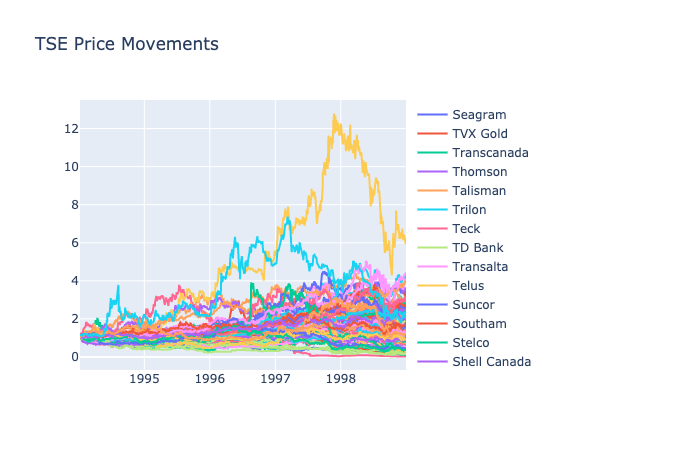
The Toronto Stock Exchange data includes a collection that may be unfamiliar to most researchers. It is a unique universe with half of the stocks decreasing in value. With a combination of both overperforming and underperforming stocks, selection strategies need to identify the ups and downs to have profitable returns.
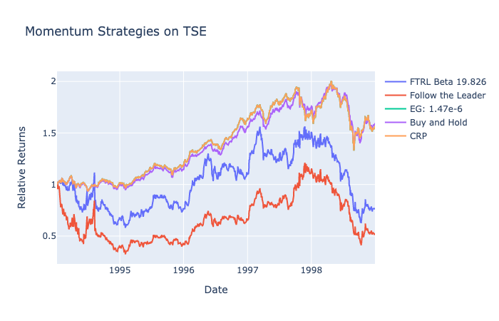
TSE’s ideal ![]() is close to 0, and ideal
is close to 0, and ideal ![]() is 19.826. A magnitude of
is 19.826. A magnitude of ![]() was necessary to lift FTRL returns, whereas
was necessary to lift FTRL returns, whereas ![]() of 0 was better for EG.
of 0 was better for EG.
The highest returns for FTRL and EG were 1.57, which was achieved by both CRP and buy and hold. Accounting for transaction cost and rebalancing, momentum strategy was ineffective for TSE as well. The presence of such a volatile but performing best stock in TSE would suggest that the momentum strategies would follow these trends. However, following the TSE price movements graph, the changes in prices are not predictive and extremely sudden. With every increase, a slight decrease follows, which represents a mean reversion trend and not a momentum one.
SP500: 1998-2003
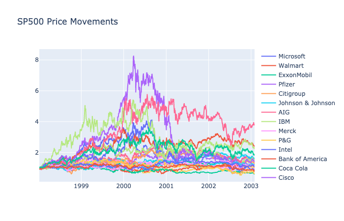
This dataset also includes the bear and bull run during turbulent times. It is longer than the DJIA data by 3 years and includes many companies that are familiar to us.
SP500 during this time goes through the bear market in 2000, and in the long run, all but 5 companies increase in value.
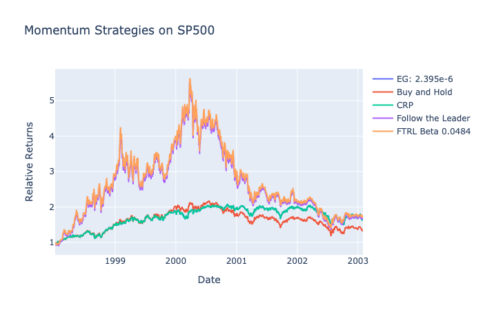
Ideal ![]() is 0, and
is 0, and ![]() is 0.048. For FTRL, we see an increase in returns for higher values of
is 0.048. For FTRL, we see an increase in returns for higher values of ![]() , and in fact, the returns for
, and in fact, the returns for ![]() of 100 is very similar to the best performing FTRL. This is in line with the results displayed below as buy and hold returned the same amount as FTRL.
of 100 is very similar to the best performing FTRL. This is in line with the results displayed below as buy and hold returned the same amount as FTRL.
SP500 during this time represents a tale of two periods. The first half has a momentum rally with FTRL returning the highest returns; however, after the peak from 2000, the portfolio rapidly decreases and converges to the rest of the strategies.
Follow the Leader, CRP, and EG all have similar returns that are marginally higher than a buy and hold, and this is another example where a lack of clear direction and continuous momentum hinders the ability to effectively predict the change in prices.
MSCI: 1993-2020
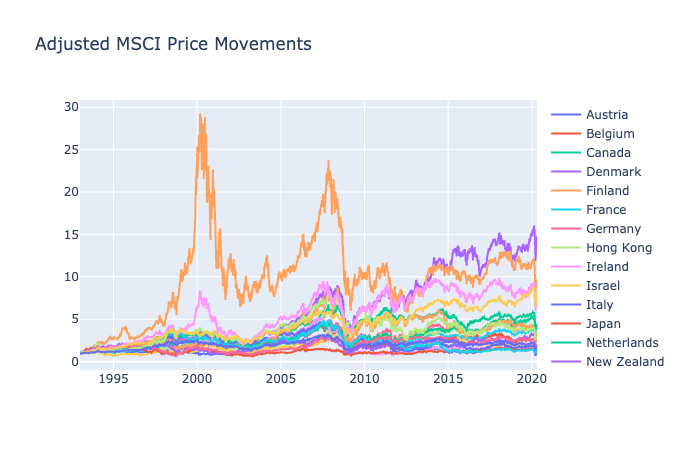
Different from traditional assets, the world indexes capture much more than just the price changes of individual companies. With an overarching representation of the countries’ market states, these market indexes will present a different idea for applications of online portfolio selection strategies.
Finland is not the first country to come in mind with metrics like these, but the rise and fall of Finland around the 2000s puts every other country aside. Most countries show movements that are strongly correlated with each other.
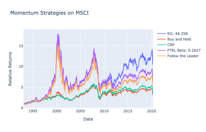
Ideal ![]() is 46.25, and
is 46.25, and ![]() is 0.2627. We see
is 0.2627. We see ![]() and
and ![]() values that are different from previous datasets. Both values indicate a measure of slight regularization to adhere to previous portfolio weights, but also emphasize the need to follow the trending asset.
values that are different from previous datasets. Both values indicate a measure of slight regularization to adhere to previous portfolio weights, but also emphasize the need to follow the trending asset.
For the MSCI dataset, we see significantly higher returns of momentum strategies near the 2000s. Primarily because of Finland’s rapid increase from the late 1990s, EG and FTL captured and put all of its weights onto Finland. If there is an asset that performs far better for a long period, momentum strategies are effective.
A higher ![]() and lower
and lower ![]() can blindly follow the performing asset and produce higher returns. However, the trend-following strategy is extremely volatile and can also create major drawbacks to the portfolio over time.
can blindly follow the performing asset and produce higher returns. However, the trend-following strategy is extremely volatile and can also create major drawbacks to the portfolio over time.
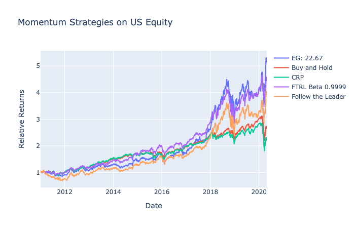
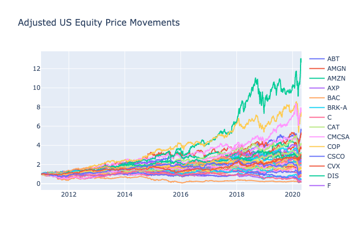
US Equity: 2011-2020
For a more recent dataset, I collected the 44 largest US stocks based on market capitalization according to a Financial Times report.
Although included in the original report, I did not include United Technologies and Kraft Foods due to M&A and also excluded Hewlett-Packard because of the company split in 2015.
This dataset will be particularly interesting because it also includes the recent market impact by the coronavirus as well. With 10 years of continuous bull run after the financial crisis in 2008, we can examine which strategy was the most robust to the rapidly changing market paradigm in the last month.
Ideal ![]() is 22.67, and
is 22.67, and ![]() is 0.9999.
is 0.9999.
For US Equity, momentum strategies also outperform buy and hold. Starting from 2018, the gap between the benchmarks becomes larger as momentum catches onto Amazon’s rapidly growing prices. There is still an insurmountable gap between Amazon’s performance and other strategies as Amazon has been performing incredibly well in the last decade. Moreover, the 10-year bull run allowed our strategies to progress well without too many drawdowns during the period.
Conclusion
Through this post, we were able to explore the momentum functionalities of PortfolioLab’s newest Online Portfolio Selection module. Readers were exposed to a basic introduction to the momentum strategies and will be able to replicate results using the simple methods of the new module.
The next post will present on Mean Reversion.
If you enjoyed reading this please leave us a star on GitHub and join our Slack channel to ask us any questions!
Online Portfolio Selection Strategies
Throughout the next couple of weeks, we will be releasing notebooks on the following strategies
- Benchmarks
- Buy and Hold
- Best Stock
- Constant Rebalanced Portfolio
- Best Constant Rebalanced Portfolio
- Momentum
- Exponential Gradient
- Follow the Leader
- Follow the Regularized Leader
- Mean Reversion
- Confidence Weighted Mean Reversion
- Passive Aggressive Mean Reversion
- Online Moving Average Reversion
- Robust Median Reversion
- Pattern Matching
- Nonparametric Histogram/Kernel-Based/Nearest Neighbor Log-Optimal
- Correlation Driven Nonparametric Learning
- Nonparametric Kernel-Based Semi-Log-Optimal/Markowitz/GV
- Meta Algorithm
- Aggregating Algorithm
- Fast Universalization Algorithm
- Online Gradient Updates
- Online Newton Updates
- Follow the Leading History
- Universal Portfolio
- Universal Portfolio
- CORN-U
- CORN-K
- SCORN-K
- FCORN-K

![NYSE Exponential Gradient Eta [0, 1]](https://hudsonthames.org/wp-content/uploads/2020/05/newplot-19.png)
![NYSE Exponential Gradient Eta [1, 100]](https://hudsonthames.org/wp-content/uploads/2020/05/newplot-1-1.png)
![NYSE Follow the Regularized Leader Beta [0, 1]](https://hudsonthames.org/wp-content/uploads/2020/05/newplot-2-1.png)
![NYSE Follow the Regularized Leader Beta [1, 100]](https://hudsonthames.org/wp-content/uploads/2020/05/newplot-9-2.png)
![DJIA Exponential Gradient Eta [0, 1]](https://hudsonthames.org/wp-content/uploads/2020/05/newplot-4-1.png)
![DJIA Exponential Gradient Eta [1, 100]](https://hudsonthames.org/wp-content/uploads/2020/05/newplot-5-1.png)
![DJIA Follow the Regularized Leader Beta [0, 1]](https://hudsonthames.org/wp-content/uploads/2020/05/newplot-6-1.png)
![DJIA Follow the Regularized Leader Beta [1, 100]](https://hudsonthames.org/wp-content/uploads/2020/05/newplot-7-1.png)
![TSE Exponential Gradient Eta [0, 1]](https://hudsonthames.org/wp-content/uploads/2020/05/newplot-9-1.png)
![TSE Exponential Gradient Eta [1, 100]](https://hudsonthames.org/wp-content/uploads/2020/05/newplot-10-1.png)
![TSE Follow the Regularized Leader Beta [0, 1]](https://hudsonthames.org/wp-content/uploads/2020/05/newplot-11-1.png)
![TSE Follow the Regularized Leader Beta [1, 100]](https://hudsonthames.org/wp-content/uploads/2020/05/newplot-12-1.png)
![SP500 Exponential Gradient Eta [0, 1]](https://hudsonthames.org/wp-content/uploads/2020/05/newplot-14-1.png)
![SP500 Exponential Gradient Eta [1, 100]](https://hudsonthames.org/wp-content/uploads/2020/05/newplot-15-1.png)
![SP500 Follow the Regularized Leader Beta [0, 1]](https://hudsonthames.org/wp-content/uploads/2020/05/newplot-16-2.png)
![SP500 Follow the Regularized Leader Beta [1, 100]](https://hudsonthames.org/wp-content/uploads/2020/05/newplot-17-1.png)
![MSCI Exponential Gradient Eta [0, 1]](https://hudsonthames.org/wp-content/uploads/2020/05/newplot-19-1.png)
![MSCI Exponential Gradient Eta [1, 100]](https://hudsonthames.org/wp-content/uploads/2020/05/newplot-20-1.png)
![MSCI Follow the Regularized Leader Beta [0, 1]](https://hudsonthames.org/wp-content/uploads/2020/05/newplot-21-1.png)
![MSCI Follow the Regularized Leader Beta [1, 100]](https://hudsonthames.org/wp-content/uploads/2020/05/newplot-22-1.png)
![US Equity Exponential Gradient Eta [0, 1]](https://hudsonthames.org/wp-content/uploads/2020/05/newplot-24-1.png)
![US Equity Exponential Gradient Eta [1, 100]](https://hudsonthames.org/wp-content/uploads/2020/05/newplot-25-1.png)
![US Equity Follow the Regularized Leader Beta [0, 1]](https://hudsonthames.org/wp-content/uploads/2020/05/newplot-26-2.png)
![US Equity Follow the Regularized Leader Beta [1, 100]](https://hudsonthames.org/wp-content/uploads/2020/05/newplot-27-2.png)
