Portfolio Optimisation with PortfolioLab: Hierarchical Risk Parity
By Aman Dhaliwal and Aditya Vyas
Join the Reading Group and Community: Stay up to date with the latest developments in Financial Machine Learning!
In 2016, Dr. Marcos Lopez de Prado introduced the Hierarchical Risk Parity (HRP) algorithm for portfolio optimization. Prior to this, Harry Markowitz’s Modern Portfolio Theory (MPT) was used as an industry-wide benchmark for portfolio optimization. MPT was an amazing accomplishment in the field of portfolio optimization and risk management, earning Harry Markowitz a Nobel Prize for his work. However, even though it is mathematically sound, it fails to produce optimal portfolios which can perform in real-world scenarios. This can be mainly attributed to two different reasons:
- It involves the estimation of returns for a given set of assets. In real life, accurately estimating returns for a set of assets is very difficult, and even small errors in estimation can cause sub-optimal performance.
- Mean-variance optimization methods involve the inversion of a covariance matrix for a set of assets. This matrix inversion makes the algorithm susceptible to market volatility and can heavily change the results for small changes in the correlations.
The HRP algorithm aims to solve some of these issues with a new approach based on the notion of hierarchy. This algorithm is computed in three main steps:
- Hierarchical Clustering – breaks down our assets into hierarchical clusters
- Quasi-Diagonalization – reorganizes the covariance matrix, placing similar assets together
- Recursive Bisection – weights are assigned to each asset in our portfolio
Throughout this post, we will explore the intuition behind HRP and also learn to apply it using the PortfolioLab library. Please keep in mind that this is a tutorial styled post and if you would like to learn more about the theory behind this algorithm, please refer to this article.
LEARN MORE ABOUT PORTFOLIO OPTIMIZATION WITH “THE MODERN GUIDE TO PORTFOLIO OPTIMIZATION”
How the Hierarchical Risk Parity algorithm works?
In this section, we will go through each step of the HRP algorithm quickly and explain the intuition behind them.
Hierarchical Clustering
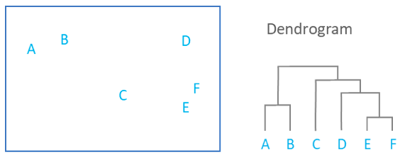
Hierarchical clustering is used to place our assets into clusters suggested by the data and not by previously defined metrics. This ensures that the assets in a specific cluster maintain similarity. The objective of this step is to build a hierarchical tree in which our assets are all clustered on different levels. Conceptually, this may be difficult for some to understand, which is why we can visualize this tree through a dendrogram.
The previous image shows the hierarchical clustering process results through a dendrogram. As the square containining our assets A-F showcases the similarity between each other, we can understand how the assets are clustered. Keep in mind that we are using agglomerative clustering, which assumes each data point to be an individual cluster at the start.
First, the assets E and F are clustered together as they are the most similar. This is followed by the clustering of assets A and B. From this point, the clustering algorithm then includes asset D (and subsequently asset C) into the first clustering pair of assets E and F. Finally, the asset pair A and B is then clustered with the rest of the assets in the last step.
So you now may be asking, how does the algorithm know which assets to cluster together? Of course, we can visually see the distance between each asset, but our algorithm cannot. There are a few widely used methods for calculating the measure of distance/similarity within our algorithm:
- Single Linkage – the distance between two clusters it the minimum distance between any two points in the clusters
- Complete Linkage – the distance between two clusters is the maximum of the distance between any two points in the clusters
- Average Linkage – the distance between two clusters is the average of the distance between any two points in the clusters
- Ward Linkage – the distance between two clusters is the increase of the squared error from when two clusters are merged
Thankfully, we can easily implement each linkage algorithm within the PortfolioLab library, allowing us to quickly compare the results to each other.
Quasi-Diagonalization
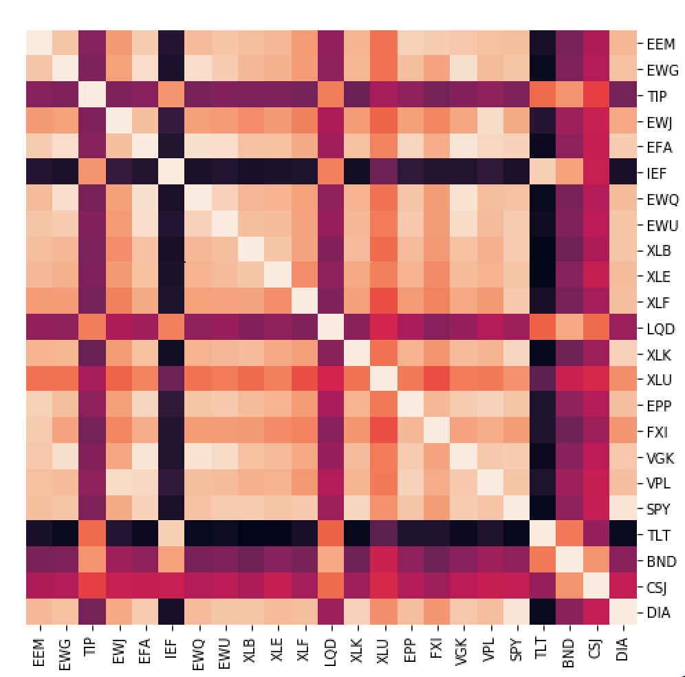
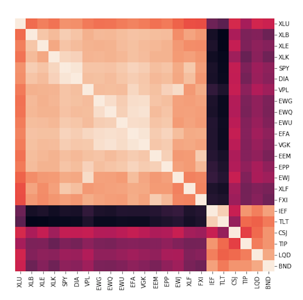
Once our assets are all clustered into a hierarchical tree, we can now perform our quasi-diagonalization step in our algorithm. From our previous step, we clustered all our assets into a hierarchical tree based on similarity defined through our chosen distance measure. In this step, we rearrange the rows and columns of the covariance matrix of assets so that we place similar assets together and dissimilar assets further apart. Once completed, this step rearranges our covariance matrix in a way so that the larger covariances in our matrix are placed along the diagonal, with the smaller ones spread around this diagonal. Because the off-diagonal elements are not completely zero, this is called our quasi-diagonal covariance matrix.
From the images shown above, we can see how the unclustered matrix shows asset clusters in small sub-sections of our matrix, while after quasi-diagonalization our clustering structure becomes much more visible.
At this point in our algorithm, all of our assets have been clustered in a hierarchical tree and our covariance matrix has been rearranged accordingly.
Recursive Bisection
Recursive bisection is the final and most important step in our algorithm. In this step, the actual portfolio weights are assigned to our assets in a top-down recursive manner.
At the end of our first step, we were left with our large hierarchical tree with one giant cluster and subsequent clusters nested within each other. By performing this step, we break each cluster into sub-clusters by starting with our largest cluster and moving down our tree in a top-down manner. Recursive bisection makes use of our quasi-diagonalized covariance matrix for recursing into the clusters under the assumption that for a diagonal matrix, the inverse-variance allocation is the most optimal allocation.
One of the main advantages to having this step in our algorithm is that our assets are only competing for weight allocation within the same cluster, leading us to developing a much more robust portfolio.
HIT THE GROUND RUNNING NOW
WITH PORTFOLIOLAB
Using PortfolioLab’s HRP Implementation
In this section, we will go through a working example of using the Hierarchical Risk Parity implementation provided by PortfolioLab and test it on a portfolio of assets.
# importing our required libraries
import pandas as pd
import numpy as np
import matplotlib.pyplot as plt
import matplotlib.patches as mpatches
from portfoliolab.clustering import HierarchicalRiskParity
Choosing the Dataset
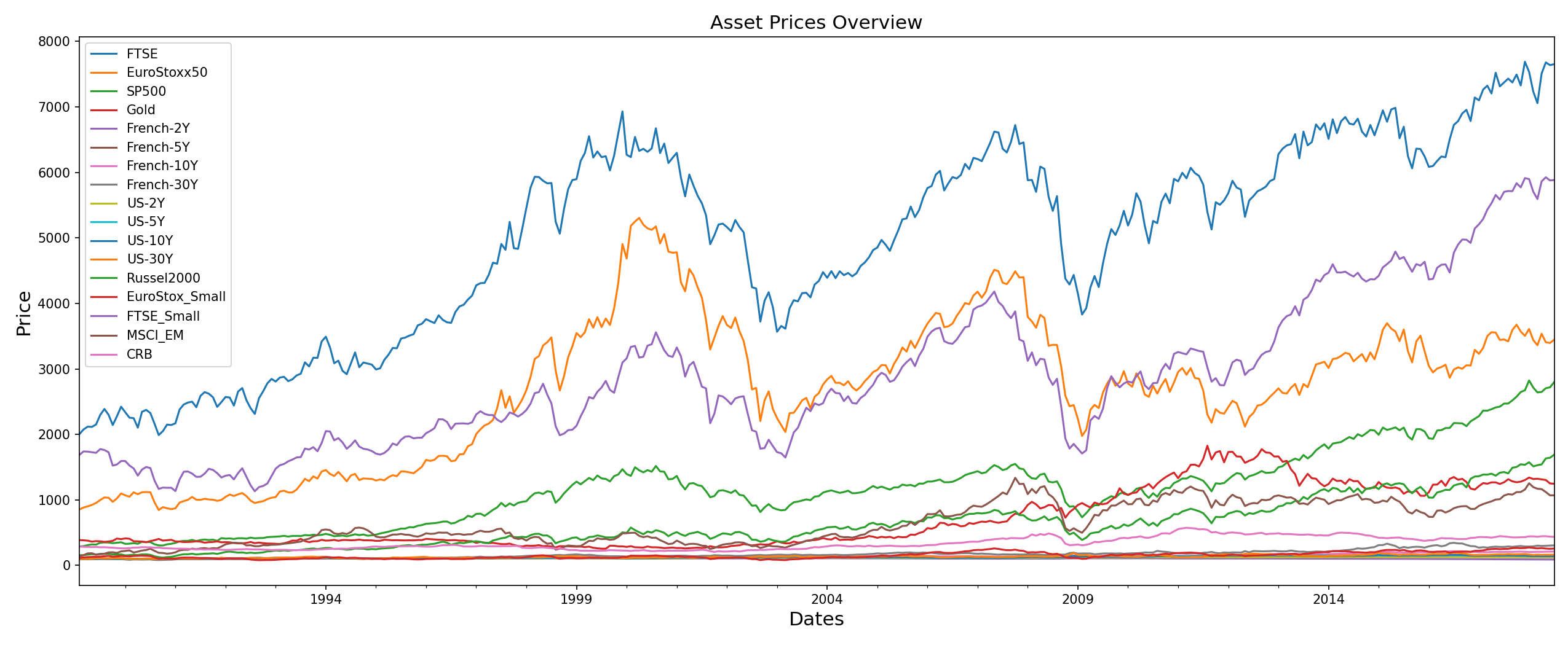
In this example, we will be working with historical closing-price data for 17 assets. The portfolio consists of diverse set of assets ranging from commodities to bonds.
# reading in our data
raw_prices = pd.read_csv('assetalloc.csv',
                         sep=';',
                         parse_dates=True,
                         index_col='Dates')
stock_prices = raw_prices.sort_values(by='Dates')
stock_prices.head()stock_prices.resample('M').last().plot(figsize=(17,7))
plt.ylabel('Price', size=15)
plt.xlabel('Dates', size=15)
plt.title('Stock Data Overview', size=15)
plt.show()
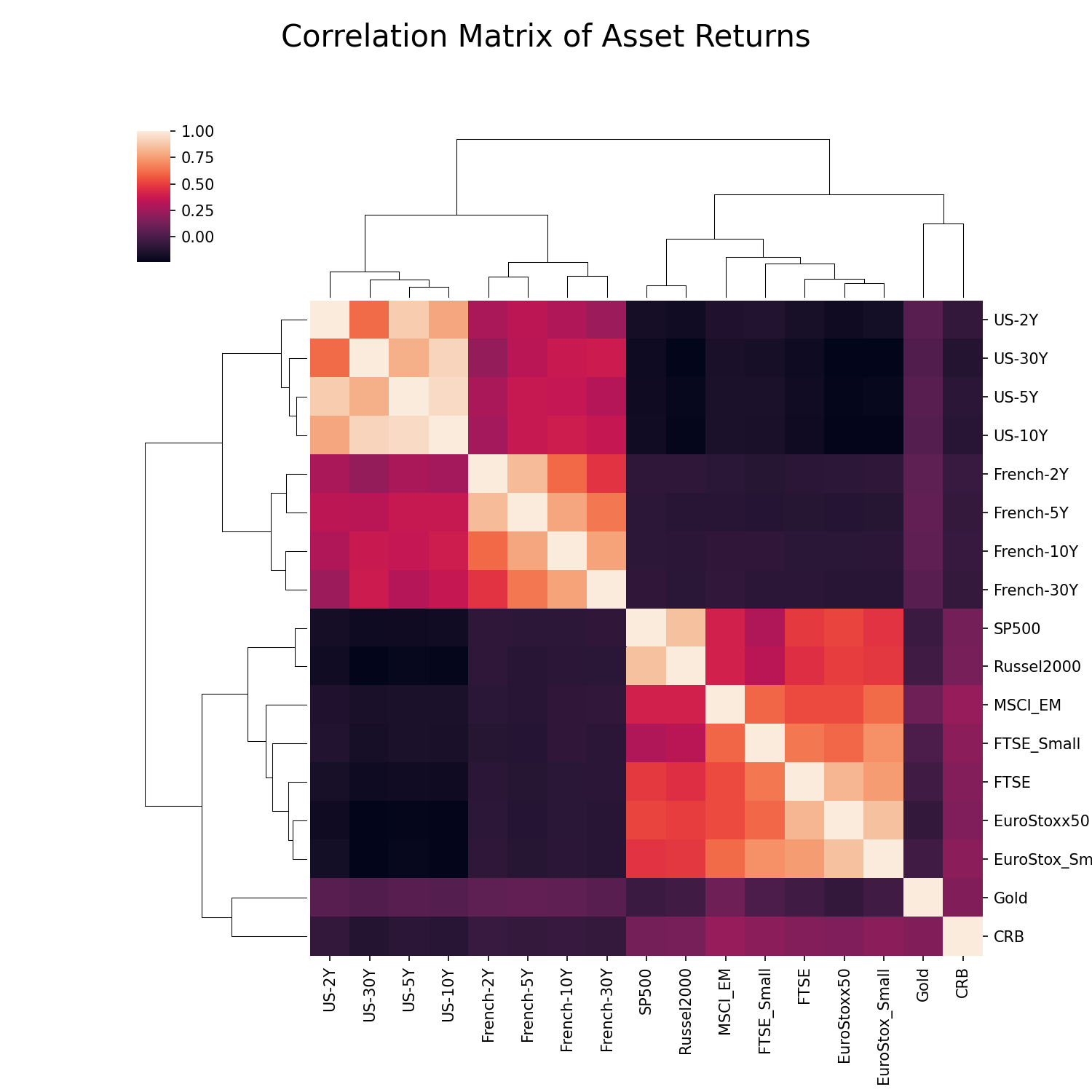
The specific set of securities have very good clustering structure which is important for hierarchical based algorithms. If you look at the visual representation of the correlation matrix below, the inherent clusters can be clearly identified. Hierarchical clustering based algorithms achieve the best performance when the data can be divided easily into clusters.
Calculating the Optimal Weight Allocations
Now that we have our data loaded in, we can make use of the HierarchicalRiskParity class from PortfolioLab to construct our optimal portfolio. First we must instantiate our class and then run the allocate() method to optimize our portfolio.
The allocate method requires only two parameters to run its default solution:
- asset_names (a list of strings containing the asset names)
- asset_prices (a dataframe of historical asset prices – daily close)
Note: The list of asset names is not a necessary parameter. If your input data is in the form of a dataframe, it will use the column names as the default asset names.
Users are also given the option to customize many different parameters in the allocate() method, some of these include:
- The type of linkage algorithm being used
- Pass a custom distance matrix
- Build a long/short portfolio
PortfolioLab currently supports all four linkage algorithms discussed in this post, although the default method described in the original HRP paper is the Single Linkage algorithm.
Additionally, instead of providing raw historical closing prices, users can choose to input their own asset returns and a covariance matrix. We will explore this in more detail later but for now, we will only be working with the two required parameters as well as specifying our linkage algorithm of choice.
# constructing our HRP portfolio - Single Linkage
hrp = HierarchicalRiskParity()
hrp.allocate(asset_names=stock_prices.columns,
             asset_prices=stock_prices,
             linkage='single')
# plotting our optimal portfolio
hrp_weights = hrp.weights
y_pos = np.arange(len(hrp_weights.columns))

plt.figure(figsize=(25,7))
plt.bar(list(hrp_weights.columns), hrp_weights.values[0])
plt.xticks(y_pos, rotation=45, size=10)
plt.xlabel('Assets', size=20)
plt.ylabel('Asset Weights', size=20)
plt.title('HRP Portfolio', size=20)
plt.tight_layout()
plt.savefig('HRP Portfolio Weights')
plt.show()
Plotting the Clusters
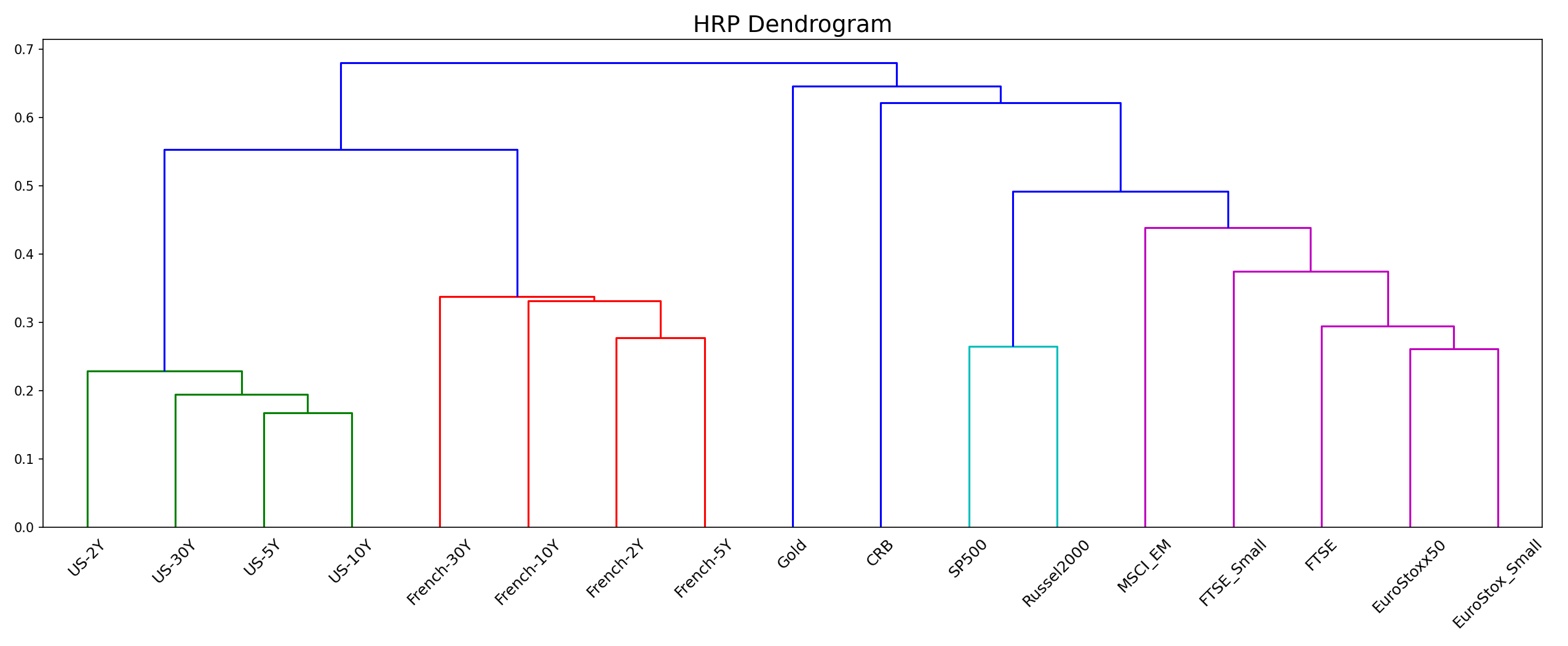
Having allocated the weights, let us look at the tree structure generated by the hierarchical clustering step. This is visualised in the form of a dendrogram as shown below.
# plotting dendrogram of HRP portfolio
plt.figure(figsize=(17,7))
hrp.plot_clusters(stock_prices.columns)
plt.title('HRP Dendrogram', size=18)
plt.xticks(rotation=45)
plt.tight_layout()
plt.show()
In this graph, the different colors of the tree structure represent the clusters that the stocks belong to.
Using Custom Input with PortfolioLab
PortfolioLab also provides users with a lot of customizability when it comes to creating their optimal portfolios. Instead of providing the raw historical closing prices for assets, users can instead input asset returns, a covariance matrix of asset returns, a distance matrix, and side weights.
In this section, we will make use of the following parameters in the allocate() method to construct a custom use case:
- asset_returns – (pd.DataFrame/numpy matrix) User supplied matrix of asset returns
- covariance_matrix – (pd.DataFrame/numpy matrix) User supplied covariance matrix of asset returns
- distance_matrix – (pd.DataFrame/numpy matrix) User supplied distance matrix
We will be constructing our first custom portfolio using the asset_returns and covariance_matrix parameters. To make some of the necessary calculations, we will make use of the ReturnsEstimators class provided by PortfolioLab.
# importing ReturnsEstimation class from PortfolioLab
from portfoliolab.estimators import ReturnsEstimators

# calculating our asset returns
returns = ReturnsEstimators.calculate_returns(stock_prices)

# calculating our covariance matrix
cov = returns.cov()

# constructing our first custom portfolio
hrp_custom = HierarchicalRiskParity()
hrp_custom.allocate(asset_names=stock_prices.columns,
                    asset_returns=returns,
                    covariance_matrix=cov)

# plotting our optimal portfolio
hrp_custom_weights = hrp_custom.weights
y_pos = np.arange(len(hrp_custom_weights.columns))

plt.figure(figsize=(25,7))
plt.bar(list(hrp_custom_weights.columns), hrp_custom_weights.values[0])
plt.xticks(y_pos, rotation=45, size=10)
plt.xlabel('Assets', size=20)
plt.ylabel('Asset Weights', size=20)
plt.title('HRP - Custom Portfolio', size=20)
plt.tight_layout()
plt.show()
You can notice we get the same weight allocations as the ones when we instead passed raw asset prices. You can use your own pre-calculated covariance matrices and asset returns or rely on our inbuilt calculation methods for calculating weights.
Passing a Custom Distance Matrix
Note that the Hierarchical Risk Parity algorithm proposed in the original paper uses the following distance matrix:
\begin{aligned}
D = \sqrt{0.5 * (1 – ⍴)}
\end{aligned}
where ![]() refers to the correlation matrix of asset returns. Users can choose to use the HRP method as it is or can tweak its performance by passing their our own distance matrix to calculate our optimal portfolio. All other steps of the algorithm will stay the same.
refers to the correlation matrix of asset returns. Users can choose to use the HRP method as it is or can tweak its performance by passing their our own distance matrix to calculate our optimal portfolio. All other steps of the algorithm will stay the same.
from portfoliolab.estimators import RiskEstimators

# create our own distance matrix
corr = RiskEstimators.cov_to_corr(cov)
distance = np.sqrt((1 - corr).round(5) / 2)

# allocate weights
hrp_distance = HierarchicalRiskParity()
hrp_distance.allocate(asset_names=stock_prices.columns,
                      distance_matrix=distance,
                      covariance_matrix=cov)

# plotting our optimal portfolio
hrp_distance_weights = hrp_distance.weights
y_pos = np.arange(len(hrp_distance_weights.columns))

plt.figure(figsize=(25,7))
plt.bar(list(hrp_distance_weights.columns), hrp_distance_weights.values[0])
plt.xticks(y_pos, rotation=45, size=10)
plt.xlabel('Assets', size=20)
plt.ylabel('Asset Weights', size=20)
plt.title('HRP - Custom Distance Matrix', size=20)
plt.show()
Building a Long-Short Portfolio
This is an extra feature we have added to our HRP implementation. By default, shorting of assets is not allowed in the original algorithm. But with PortfolioLab’s implementation, you can pass a side_weights parameter to short some assets in your portfolio.
In the following example, we will short the first four stocks in our dataset. All other steps remain the same – the only difference being the addition of the side_weights parameter to indicate which stocks we would like to short and long (-1 indicates shorting a stock and 1 indicates going long on a stock).
side_weights = pd.Series([1]*stock_prices.shape[1], index=stock_prices.columns)

# short the first 4 stocks
side_weights.loc[stock_prices.columns[:4]] = -1

print(side_weights)
FTSE             -1
EuroStoxx50      -1
SP500            -1
Gold             -1
French-2Y         1
French-5Y         1
French-10Y        1
French-30Y        1
US-2Y             1
US-5Y             1
US-10Y            1
US-30Y            1
Russel2000        1
EuroStox_Small    1
FTSE_Small        1
MSCI_EM           1
CRB               1
dtype: int64
# calculating optimal weights
hrp_ls = HierarchicalRiskParity()
hrp_ls.allocate(asset_names=stock_prices.columns,
                asset_prices=stock_prices,
                side_weights=side_weights)

# plotting our optimal portfolio
hrp_ls_weights = hrp_ls.weights
y_pos = np.arange(len(hrp_ls_weights.columns))

plt.figure(figsize=(25,7))
plt.bar(list(hrp_ls_weights.columns), hrp_ls_weights.values[0])
plt.xticks(y_pos, rotation=45, size=10)
plt.xlabel('Assets', size=20)
plt.ylabel('Asset Weights', size=20)
plt.title('HRP - Long/Short Portfolio', size=20)
plt.tight_layout()
plt.savefig('HRP Long-Short Portfolio')
plt.show()
Conclusion and Further Reading
Through this post, we learned the intuition behind the Hierarchical Risk Parity algorithm and also saw how we can utilize PortfolioLab’s implementation to apply this technique out-of-the-box. HRP is a powerful algorithm that can produce robust risk-parity portfolios which avoids many of the limitations of traditional mean-variance optimisation methods.
The following links provide a more detailed exploration of the algorithm for further reading.

