Sparse Mean-reverting Portfolio Selection

by Yefeng Wang

Join the Reading Group and Community: Stay up to date with the latest developments in Financial Machine Learning!

Introduction

“Buy low, sell high.” One cannot find a more succinct summary of a mean-reversion trading strategy; however, single assets that show stable mean-reversion over a significant period of time such that a mean-reversion trading strategy can readily become profitable are rare to find in markets today. Even if such gems were found, celebrating the discovery of the gateway to easy money could prove premature:

The asset may exhibit low volatility and the gap between the extreme prices of the asset and its long-term mean is too small. In this case, you can either try trading large size to capture enough profit with your risk desk’s consent (good luck with that) or do not bother with it at all.
The asset is hard to short-sell. Either due to regulatory restrictions or unexpected events, not being able to short-sell at the most opportune moment can significantly affect the profitability of the strategy.
The mean-reversion occurs at a time scale of months or even years. In this case, you might as well try a momentum strategy on a shorter time scale instead of carrying out the mean-reversion strategy to a T.

Looks like searching for a magic asset that possesses perfect mean-reversion is impractical. Instead, building tradable mean-reverting long-short portfolios whose value is the weighted aggregate price of a basket of assets has become the focus of statistical arbitrageurs. The simplest form of this type of portfolios is an asset pair, and I have discussed in my previous article how to find such asset pairs using the concept of cointegration in detail. This article, on the other hand, extends the discussion into the territory of multi-asset (reads more than two assets) sparse mean-reverting portfolio selection.

“Why do I even need this new methodology? I can assemble multiple cointegrated pairs into a multi-asset mean-reverting portfolio anyway.”

This is definitely feasible thanks to machine learning, but it could become confusing to build the portfolio if the pairs have overlapping legs. Say your favorite pair selection black box spits out a list of candidate mean-reverting asset duos whose spread value is stationary. One of these pairs longs asset A and shorts asset B, while another one longs asset C and shorts asset A. Now the ambiguity kicks in. Since both these pairs are stationary, any linear combination of them will stay stationary as well. There are theoretically infinite possibilities and it would become a nightmare scenario for decision-making when the number of overlapping pairs increases. Therefore, a multi-asset oriented methodology that can give more definitive solutions is preferred.

“OK. Sounds fair. So how many assets are adequate for such a mean-reverting portfolio?”

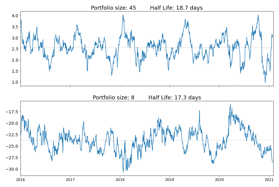
Now we’re rolling! Let’s see an example first (Footnote 1).

Figure 1. Two portfolios with similar mean-reversion properties but trading different number of assets.

Obviously, these two portfolios have similar mean-reversion properties. However, the first portfolio requires us to trade 45 assets, while the second one only requires eight! I would choose the second portfolio without a doubt as it is easier to manage, its P&L is more straightforward to interpret, and fewer assets means lower transaction costs. Sounds like winning! Therefore, the answer to the previous question is: while there are no strict rules for the exact number of assets to include in the portfolio, it is preferable to have as few assets as possible.

So how should we build the ideal multi-asset mean-reverting portfolio? As you are grabbing the snacks and water for the treasure hunt, I’ll present you the treasure map:

The article follows very closely to the work of d’Aspremont (2011) and Cuturi and d’Aspremont (2015), so make sure you download these two papers from the reference section at the end of this article as well. If you prefer watching a video instead of reading an article, I’ve got you covered as well.

Let’s now get to it!

You need to quantify what you want to optimize

Let’s recapitulate the objective:

The portfolio, i.e. the linear combination of the assets, should be strongly mean-reverting.
The portfolio should be sparse, i.e. having more than two assets but not too many in the meantime.

Computers will not be able to understand qualitative descriptions such as “strongly mean-reverting” and “not too many assets”, but these two quantities are the crux of finding a solution to this portfolio selection problem.

The “not too many assets” condition is straightforward. Suppose there are $n$ assets in total in the investment universe, and we can simply set the number of assets to an integer $k$ , where $k << n$ ; for example, we can set $k = \lfloor 0.1n \rfloor$ . Then what about “strongly mean-reverting”? How should we measure strength of mean-reversion of a time series?

Metrics to measure mean reversion strength

Assuming the value of the mean-reversion portfolio follows an Ornstein-Uhlenbeck (OU) process (for more details on Ornstein-Uhlenbeck processes, check out our previous article or the wonderful book Optimal Mean reversion Trading: Mathematical Analysis and Practical Applications by Prof. Tim Leung and Xin Li (2015)):

$d\Pi_t = \lambda(\bar{\Pi} - \Pi_t)dt + \sigma dZ_t$
$\Pi_t = \sum_{i=1}^n x_i S_{ti}$
$\lambda > 0$

where $\Pi_t$ is the value of the portfolio at time $t$ , $\bar{\Pi}$ is the long term mean level of the portfolio value, $S_{ti}$ is the value of an asset $S_i$ at time $t$ , $x_i$ is the weight for asset $S_i$ , $\sigma$ is the instantaneous volatility, $Z_t$ is a standard Brownian motion, and the parameter $\lambda$ is the mean reversion speed.

“Woah, slow down with the math!” You started rubbing your eyes. “Wait… Isn’t this mean reversion speed parameter $\lambda$ the metric we are looking for? The faster the mean reversion speed, the stronger the mean reversion. Problem solved!”

Indeed, with the introduction of $\lambda$ , we can now formulate our sparse portfolio selection problem in more precise mathematical language:

$\text{maximize } & \lambda$
$\text{subject to } & \lVert x \rVert_0 = k$

where $\lVert x \rVert_0$ is the cardinality, or the $l_0$ norm (both reads the number of non-zero elements) of the asset weighting vector $x$ .

Say we find a weighting vector $y$ that formed a portfolio with a reasonably high $\lambda$ value. How do we know $y$ is the optimal solution? If $y$ is not the optimal solution, in which direction should we search for a better weighting? It is hard to answer these questions without a well-defined function between $\lambda$ and $x$ .

Other proxies of mean reversion strength

The moment of joy was evanescent. The problem still looks difficult to solve. But not all hopes are lost. The OU mean reversion speed parameter $\lambda$ is not the only mean reversion strength metric available. Cuturi and d’Aspremont (2015) introduced three mean reversion strength proxies that make the above optimization problem easier.

Predictability and Box-Tiao canonical decomposition

Suppose that the portfolio value $\Pi$ follows the recurrence below:

$\Pi_t = \hat{\Pi}_{t-1} + \varepsilon_t$

where $\hat{\Pi}_{t-1}$ is the predicted value of $\Pi_t$ based on all the past portfolio values $\Pi_0, \, \Pi_1, \, \ldots \Pi_{t-1}$ , and $\varepsilon_t \sim N(0, \Sigma)$ is a vector of i.i.d Gaussian noise independent of all past portfolio values up to $t-1$ .

Now let $\text{var}(\Pi_t) = \sigma^2$ , $\text{var}(\hat{\Pi}_{t-1}) = \hat{\sigma}^2$ , and by definition we know $\text{var}(\varepsilon_t) = \Sigma$ .

Therefore,

$\text{var}(\Pi_t) = \text{var}(\hat{\Pi}_{t-1} + \varepsilon_t) = \text{var}(\hat{\Pi}_{t-1}) + \text{var}(\varepsilon_t)$

The second equal sign stands due to the independence between $\hat{\Pi}_{t-1}$ and $\varepsilon_t$ .

Substitute in the variance, we get:

$\sigma^2 = \hat{\sigma}^2 + \Sigma$

$1 = \frac{\hat{\sigma}^2}{\sigma^2} + \frac{\Sigma}{\sigma^2}$

The predictability is then defined as

$\nu := \frac{\hat{\sigma}^2}{\sigma^2}$

The intuition behind this variance ratio is straightforward. If $\nu$ is small, then this means the Gaussian noise is the dominant force and the portfolio value will look like pure noise, which is desirable as the noise is stationary and highly mean-reverting. However, when $\nu$ is large, the portfolio value is almost perfectly predictable based on its past information and this usually leads to a momentum portfolio. Therefore, we want to minimize $\nu$ to obtain a mean-reverting portfolio.

The remaining question is to derive the estimate $\hat{\Pi}_{t-1}$ and its variance $\hat{\sigma}^2$ . Assumptions have to be made in order to get a tractable solution of the estimate. Remember that the portfolio is a linear combination of assets, i.e., $\Pi_t = x^T S_t$ , according to the notation in the previous section. Without loss of generality, we will assume that each asset price $S_{ti}$ is centered to zero mean before the analysis.

Box and Tiao (1977) proposed that the asset prices $S_t$ could be assumed to follow a vector autoregressive model of order one – a VAR(1) model. Under this assumption, the predictability can be represented by covariance matrix of $S_t$ , denoted by $\Gamma_0$ , and the least square estimate of the VAR(1) coefficient matrix $A$ :

$\nu = \frac{x^T A \Gamma_0 A^T x}{x^T \Gamma_0 x}$

Curious readers can refer to d’Aspremont (2011) and Cuturi and d’Aspremont (2015) to jostle your brain.

Let’s see how the optimization problem looks now that we have an expression of $\nu$ .

$\text{minimize } & \nu = \frac{x^T A \Gamma_0 A^T x}{x^T \Gamma_0 x}$
$\text{subject to } & \lVert x \rVert_0 = k$

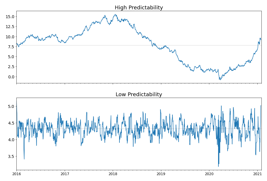
This is looking much nicer. In fact, this minimization problem without the cardinality constraint is a generalized eigenvalue problem (Ghojogh, 2019) that can be solved with ease with SciPy, and the minimum is achieved when $x$ is the eigenvector corresponding to the smallest eigenvalue. Let’s see an example of a portfolio of low predictability and one of high predictability.

Figure 2. A comparison of a highly predictable portfolio to a barely predictable portfolio.

It is apparent that the more predictable portfolio seems a great candidate for momentum strategies, while the less predictable portfolio looks very much like noise and highly mean-reverting (and perhaps too noisy to trade). This suggests that substituting the OU-model mean-reversion speed with predictability is a move towards the right direction.

Portmanteau and crossing statistics

Before we move onto the next part, two other proxies for measuring mean-reversion strength are worth noting.

Portmanteau statistic

The portmanteau statistic of Ljung and Box (1978) is used to test whether a process is white noise. For our portfolio process $\Pi_t$ , denote the lag- $k$ autocovariance matrix of the asset prices $S_t$ by $\Gamma_k$ , the portmanteau statistic can be written as

$\hat{\phi}_p(x) = \frac{1}{p} \sum_{i=1}^p \Big( \frac{x^T \Gamma_i x}{x^T \Gamma_0 x} \Big)^2$

The smaller the portmanteau statistic, the stronger the mean-reversion.

Crossing statistic

Kedem and Yakowitz (1994) define the zero crossing rate of a univariate process $s_t$ , i.e. the expected number of crosses around 0 per unit of time, as

$\gamma(x) = E\Bigg[ \frac{\sum_{t=2}^{T}\mathbf{1}_{\{s_t s_{t-1 }\leq 0 \} }}{T-1} \Bigg]$

The larger the crossing statistic, the stronger the mean reversion.

Directly optimizing this statistic is difficult. However, if we assume that $s_t$ follows a stationary AR(1) process, then the zero crossing rate can be simplified using the cosine formula:

$\gamma(x) = \frac{\text{arc cos}(a)}{\pi}$

where $a$ is the AR(1) coefficient, or the first-order autocorrelation. The stationarity implies $\lvert a \rvert < 1$ , therefore, the smaller the first-order autocorrelation, the larger the crossing statistic. This result can be readily extended to the multivariate case, where we minimize the first-order autocorrelation and keep all absolute higher order autocorrelations small.

Sparse is NP-Hard

We have figured out the objective function to optimize, which is predictability. Now it is time to focus on the sparsity constraint.

“How hard can that be?” You murmured to yourself. “As the old saying goes, ‘code first, optimize later’. Let’s try brute force search first.”

For the sake of demonstration, let’s say the goal is to build a 5-asset portfolio from 30 candidate assets.

“Fine. 30 choose 5… is 142,506. Wait, this is going to take a while to enumerate every one of them.”

Now suppose we want to do the same thing but with all 505 S&P 500 constituents.

“505 choose 5… This is impossible!” (Footnote 2)

Indeed, once the cardinality constraints has been added, the easy-to-solve generalized eigenvalue problem suddenly became a hard combinatorial problem, and Natarajan (1995) has shown that it is equivalent to subset selection, which is NP-hard. This means there is no algorithm with polynomial running time that can yield the optimal solution.

However, financial practitioners are usually not perfectionists. A sub-optimal sparse portfolio that has decent mean-reversion strength is preferable if it costs much less computing power. The remainder of this article will focus on a few different approaches to getting good approximate solutions that ensure the sparsity of the portfolio.

Narrow down the investing universe

Let’s get back on the challenge of building a 5-asset portfolio from 30 candidate assets. Suppose that after analyzing the intrinsic structure of the asset price processes, we managed to find three clusters of assets, each of which contains 8 assets; and 6 isolated assets with their idiosyncrasies. Instead of examining all possible 5-asset combinations from 30 assets, we only consider the combinations within the clusters. Time to do some counting:

$\binom{30}{5} = 142,506$
$3 \times \binom{8}{5} = 168$
$\frac{142,506}{168} = \textbf{848.25}$

A computation reduction by a factor of 848.25! This is now even manageable for a brute-force search algorithm.

The immediate advantage of adding a preprocessing step has naturally led to the question: “how should we do this?” While the instinctive reaction would be machine learning, I would like to introduce something rather vanilla in flavor – the family of Least Absolute Shrinkage and Selection Operators (Lasso) and their application in covariance selection and structured VAR model estimation.

Covariance selection

The inverse covariance matrix, $\Gamma_0^{-1}$ , is a wealth of information on the dependencies of the asset price data. Under the assumption of a Gaussian model, zeroes in $\Gamma_0^{-1}$ are indicators of conditional independence between variables, which reflects “independence between the idiosyncratic components of asset price dynamics.” (d’Aspremont, 2011) Therefore, if we are able to set a reasonable portion of elements in $\Gamma_0^{-1}$ to zeroes, the remaining elements can represent the underlying structure of the asset price dependencies.

“Structure? What structure? You can’t possibly expect me to see some fascinating structure just by staring at a matrix as if I am in the Matrix!”

Don’t worry, the visualization is on its way. Note that covariance matrix $\Gamma_0$ is a symmetric matrix, hence its inverse $\Gamma_0^{-1}$ is also symmetric. This means we can use an undirected graph to represent the underlying structure of asset price dynamics. Each asset can be represented as a vertex. The non-zero element indicates an edge exists between two nodes depending on its position. The sparse estimate was obtained by graphical Lasso model, which solves a penalized maximum likelihood estimation problem:

$\max_X \, \ln \det X - \mathbf{Tr}(\Sigma X) - \alpha \lVert X \rVert_1$

$\alpha > 0$ is a parameter which determines how many zero elements there will be in the final sparse estimate. The larger $\alpha$ is, the more elements will be penalized to zero, hence the sparser the estimate.

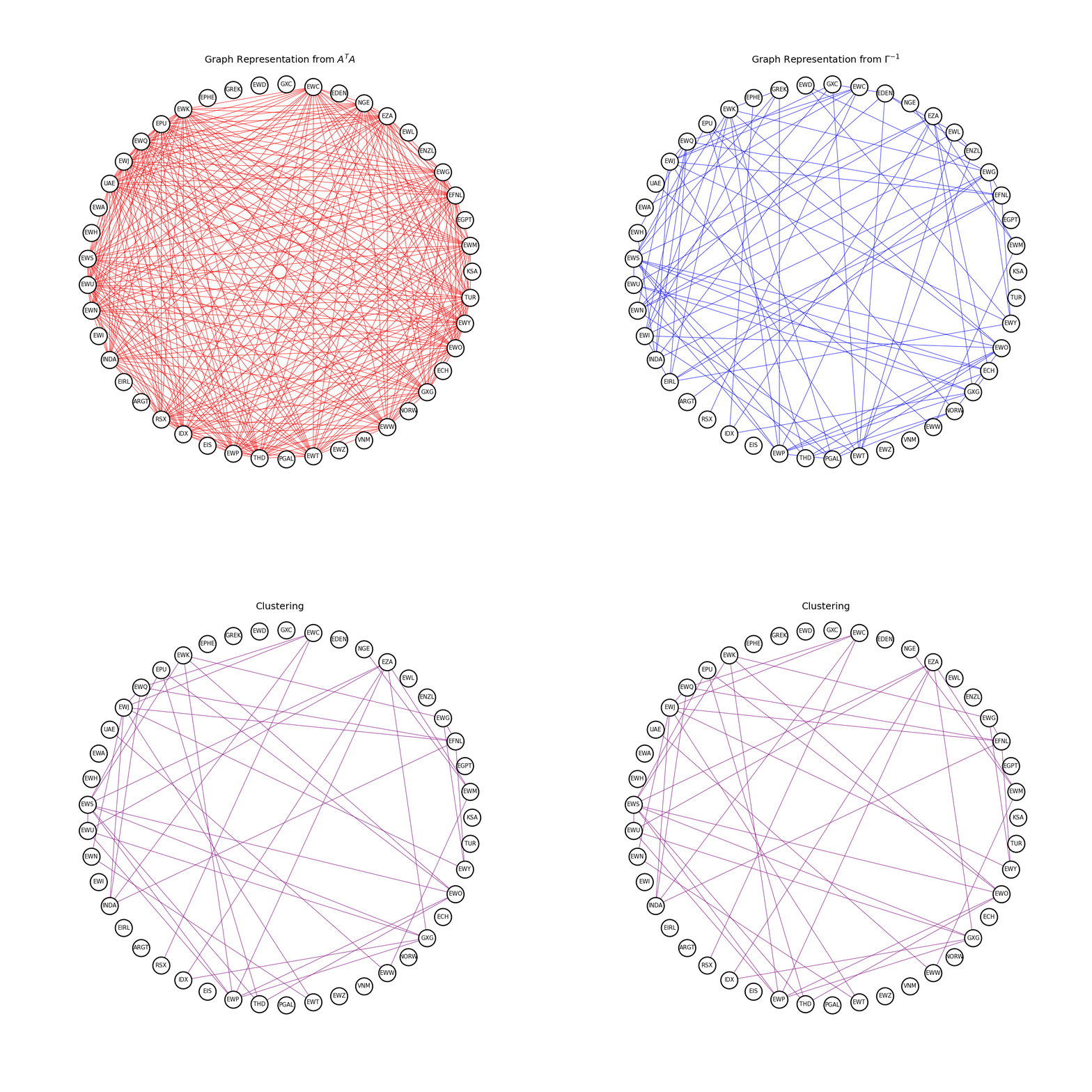
Let’s now compare the graph obtained from a dense covariance estimate and a sparse estimate. By gradually increasing $\alpha$ from 0.6 to 0.9, the edges are quickly eliminated and the final estimate are quite sparse.

Figure 3. Covariance selection at work. The graph is a representation of the inverse covariance matrix $\Gamma_0^{-1}$ .

What about the covariance matrix itself?

Figure 4. Covariance matrix obtained from the covariance selection procedure. Most matrix elements have been reduced to 0 as $\alpha$ increases.

It’s super effective! However, to obtain the smaller clusters, we still need another puzzle piece, which is a structured VAR model estimate.

Structured VAR estimate

Recall the assumption that the asset prices $S_t$ follow a VAR(1) model:

$S_t = S_{t-1} A + Z_t$

where $S_{t-1}$ is the lag-one process of $S_t$ , and $Z_t \sim N(0, \Sigma)$ is an i.i.d Gaussian noise independent of $S_{t-1}$ . The dense least square estimate of $A$ is then obtained by minimizing the objective function:

$\text{arg min}_A \, \lVert S_t - S_{t-1} A \rVert^2$

Adding an $\ell_1$ -norm penalty to the objective function will make $A$ sparse. The power of Lasso lies in that we can append different forms of $\ell_1$ -norm to exert control on the final structure of the sparse estimate of $A$ . We can either apply a univariate Lasso column-wise and optimize the following objective function $n$ times:

$\text{arg min}_{a} \, \lVert S_{it} - S_{t-1}a \rVert^2 + \lambda \lVert a \rVert_1 \text{ for all } i$

Or we can apply multi-task Lasso and get the sparse estimate of $A$ in one go by optimizing the following objective function:

$\text{arg min}_{A} \, \lVert S_{t} - S_{t-1}A \rVert^2 + \lambda \sum_i \sqrt{\sum_j a_{ij}^2}$

where $a_{ij}$ is the elements in matrix $A$ .

Figure 5 and 6 demonstrated how the structure of $A$ will evolve as we increase the regularization parameter $\lambda$ under two different $\ell_1$ -norm penalties. As you can see, the multi-task Lasso will suppress the coefficients in an entire column to zero, but the solution will become less robust as $\lambda$ increases. The univariate Lasso applied column-wise, on the other hand, will lead to a much more scattered structure but more stable.

Figure 5. Univariate Lasso applied column-wise for structured VAR(1) estimate.

Figure 6. Multi-task Lasso applied column-wise for structured VAR(1) estimate.

Lock in the clusters using both sparse estimates

Both the inverse covariance matrix $\Gamma_0^{-1}$ and the VAR(1) coefficient matrix $A$ contains the conditional dependence structure of the asset price dynamics. If we can combine the information from both matrices, we can further pinpoint the clusters from which we can build our sparse mean-reverting portfolio.

While $\Gamma_0^{-1}$ has a readily available undirected graph representation, $A$ does not have one due to its asymmetry. If we can find a way to construct an undirected graph representation for $A$ , the intersection between the graph of $\Gamma_0^{-1}$ and $A$ will highlight the asset clusters we are looking for.

Gilbert (1994) has shown that if the covariance matrix of the i.i.d. Gaussian noise $Z_t$ in the VAR(1) model is diagonal, then the graph of $\Gamma_0^{-1}$ and $A^T A$ will share the identical block-diagonal structure. The important takeaway from this result is that we can use $A^T A$ , which is perfectly symmetric, as the graph representation for conditional dependence structure.

Now we can wrap up our preprocessing procedure as all necessary information has been gathered.

Use graphical Lasso to get a sparse estimate of the covariance matrix $\Gamma_0$ . Apply a sufficiently large regularization parameter to break down the graph of $\Gamma_0^{-1}$ into small clusters.
Use column-wise univariate Lasso or multi-lask Lasso to get a sparse estimate of the VAR(1) coefficient matrix $A$ . Calculate the graph representation $A^T A$ .
Retrieve the intersection graph of $\Gamma_0^{-1}$ and $A^T A$ .
The connected components of the intersection graph are the clusters we are looking for.

Figure 7. The clustering process.

In practice, successful clustering is highly dependent on covariance selection rather than the structured VAR(1) estimate. It is thus recommended to set a large regularization parameter for the graphical Lasso model for a highly sparse covariance matrix estimate (but of course you don’t want to eliminate all the edges in the graph!)

Construct a sparse solution

Recall that our portfolio selection problem has been formulated as:

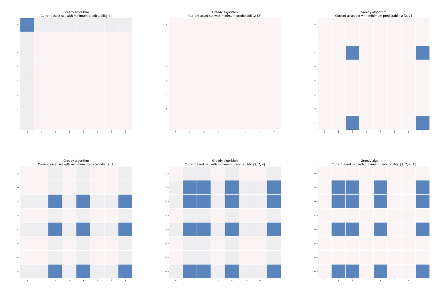
$\text{minimize } & \nu = \frac{x^T A \Gamma_0 A^T x}{x^T \Gamma_0 x}$

$\text{subject to } & \lVert x \rVert_0 = k$

A quick-and-dirty sub-optimal solution can be built from scratch with a greedy algorithm. Let’s watch an animated example instead of resorting to math again.

Figure 8. An animated explanation of the greedy algorithm.

The key idea here is to construct the portfolio recursively. At the start of the algorithm, we haven’t selected any asset into our portfolio and thus the portfolio has zero predictability. At $k$ -th iteration, we look to add the asset that leads to the smallest increase in the portfolio predictability by solving the generalized eigenvalue problem $n-k$ times for each possible asset choice as shown in Figure 8.

Why is greedy algorithm much faster? Because we ignored many candidate portfolios. Let’s say we found an $m$ -asset ( $m < k$ ) portfolio $\Pi_a$ with minimal predictability. Now if we want to add one more asset, we will not calculate the predictability for all possible portfolios with $m + 1$ assets. Rather, we will build the portfolio based on $\Pi_a$ . This effectively reduced the number of portfolios under examination from $\binom{n}{m+1}$ to $n-m$ , which is a huge improvement.

The efficiency comes with a tradeoff. Since so many candidate portfolios are not even considered, the solution given by the greedy algorithm might be far-from-optimal. Following the example in Figure 8, once the greedy algorithm selected Asset #2, it will keep building the portfolio based on this first selection. However, the optimal portfolio might not contain Asset #2 at all if we comb through every possible portfolio. This may sound like a serious disadvantage, but Fogarasi (2012) tested with simulated data and found that brute force search was able to produce a stronger mean-reversion portfolio than the greedy algorithm only 59.3% of the time. In other words, brute force search guarantees the optimal solution while greedy algorithm does not; but approximately four out of ten times, the greedy algorithm will generate the exact solution as brute force search while saving huge amount of computing time. Greed is good indeed!

Relax the constraints

The cardinality constraint $\lVert x \rVert_0 = k$ is the culprit for all the headaches so far because it made the portfolio selection problem non-convex. Here, the concept “convex” means “when an optimal solution is found, then it is guaranteed to be the best solution”, which is quite different from the fearful sense related to notorious derivatives trading debacles.

There are already a handful of tools for solving convex problems, but they are not directly portable to non-convex ones that have potentially many local optima or saddle points. Disappointing, innit? Not exactly. An eureka moment is right around the corner.

What if we loosen the non-convex cardinality constraint to a convex counterpart? Of course, the optimization problem will have changed drastically when we change the constraints, and the optimal solution for the new problem is not necessarily the optimal solution for the original one; but again, we will happily offer optimality for computational speed.

You may have wondered why I have been constantly referring to the cardinality as $\ell_0$ -norm in this article, and here is the reason:

$\ell_1$ -norm is the convex counterpart of the $\ell_0$ -norm constraint.

This is an oversimplification of the relaxation technique, but helpful for building intuition nonetheless. So how does our optimization problem look like after the convex relaxation?

Instead of working with the weighting vector $x$ , we will now work with the semidefinite matrix $X = x x^T$ (Lovász and Schrijver, 1991). The portfolio selection problem can be rewritten as:

$\text{minimize } & \mathbf{Tr} (A \Gamma_0 A^T X) / \mathbf{Tr} (\Gamma_0 X)$
$\text{subject to } & \lVert X \rVert_1 \leq k$
$& \mathbf{Tr} (X) = 1$
$& X \succeq 0$

The $l_1$ norm $\lVert X \rVert_1$ is simply the sum of the absolute value of all elements in the symmetric matrix $X$ . The extra constraint $\mathbf{Tr} (X) = 1$ is equivalent to normalizing the weighting vector $x$ to a unit vector. This could help with numerical stability. While the constraints are convex, the objective function is only quasi-convex because it is a ratio of two matrix traces, and thus cannot be readily solved by convex optimization methods.

There are two ways to get around this issue. One approach is to do a clever change of variables, and the above optimization problem can be solved via semidefinite programming (SDP). I will leave out the mathematical legerdemain and refer you to d’Aspremont (2011) for details, for this method has not been able to generate consistent results in experience despite it retained the flavor of the original optimization problem. Specifically, the cardinality parameter $k$ did not bear its supposed meaning because the optimal $X^*$ was almost never a rank-one matrix in real application, and the leading eigenvector of $X^*$ in most cases had higher cardinality than expected. We could derive the sparse leading eigenvector of $X^*$ with exactly $k$ non-zero weights using the truncated power method (Yuan and Zhang, 2013), but the resulting portfolios would take months to mean-revert, which is undesirable.

The other approach is to rewrite the optimization problem with a $\ell_1$ -norm penalty following Cuturi and d’Aspremont (2015):

$\text{minimize } & \mathbf{Tr} (A \Gamma_0 A^T X) + \rho \lVert X \rVert_1$
$\text{subject to } & \mathbf{Tr} (\Gamma_0 X) \geq V$
$& \mathbf{Tr} (X) = 1$
$& X \succeq 0$

Comparing to the original objective function $\mathbf{Tr} (A \Gamma_0 A^T X) / \mathbf{Tr} (\Gamma_0 X)$ , this formulation focuses on minimizing the numerator of the ratio while keeping the denominator above a threshold. The addition of the $\ell_1$ -norm penalty introduces sparsity. Everything makes sense mathematically, but are there any applicable financial interpretations?

The answer is a resounding yes. Note that the term $\mathbf{Tr}(\Gamma_0 X)$ represents the variance of the portfolio and the constraint guarantees that the variance exceeds $V$ . This optimization problem is de facto minimizing portfolio predictability while ensuring the portfolio value has sufficient volatility! We also made sure that not too many assets are included in the portfolio with the $\ell_1$ -norm penalty. But wait, there’s more: this formulation can be used to optimize portmanteau and crossing statistic as well!

The only drawback of this approach is that the cardinality is no longer clearly defined as it is determined by the $\ell_1$ -regularization parameter $\rho$ , which means a bit more tweaks are required to achieve the desired cardinality, but we can’t really complain as the flexibility and interpretability we have gained via this formulation far outweighs the minor inconvenience.

Compared to the cut-to-the-chase greedy algorithm, the convex relaxation approach is more complicated in terms of theory and time complexity, but its versatility allows more control over the behavior of the portfolio. Curious readers can refer to Cuturi and d’Aspremont (2015) for a deep-dive into the application of convex relaxation approach to solving the sparse mean-reverting portfolio problem.

LEARN MORE ABOUT PAIRS TRADING STRATEGIES WITH “THE DEFINITIVE GUIDE TO PAIRS TRADING”

READ NOW

Talk is cheap, show me the results!

I am extremely impressed if you are still with me from the start, as I have already fatigued myself from explaining all the theories. Now let’s see how ArbitrageLab can simplify the sparse mean-reverting portfolio construction process with a few line of codes. Supposedly, the data have already been properly processed and all missing values have been imputed. Since the ETF data was used for demonstration (Footnote 1), I will assume the price data has already been saved in the variable etf_df.

Asset Clustering

In the previous section, I discussed how to use sparse estimates of covariance matrix and VAR(1) coefficient matrix to find smaller asset clusters. Box-Tiao canonical decomposition can be then applied to the small cluster to get a sparse mean-reverting portfolio. This can be readily done with ArbitrageLab.

from arbitragelab.cointegration_approach.sparse_mr_portfolio import SparseMeanReversionPortfolio
import networkx as nx

etf_sparse_portf = SparseMeanReversionPortfolio(etf_df)

# Calculate the penalized estimates
sparse_var_est = etf_sparse_portf.LASSO_VAR_fit(1.4, threshold=7, multi_task_lasso=True,
                                                use_standardized=True)
_, sparse_prec_est = etf_sparse_portf.covar_sparse_fit(0.89, use_standardized=True)

# Generate the clusters
multi_LASSO_cluster_graph = etf_sparse_portf.find_clusters(sparse_prec_est, sparse_var_est)

# Initialize a new class instance with the smaller cluster
small_cluster = list(sorted(nx.connected_components(multi_LASSO_cluster_graph), 
                            key=len, reverse=True))[1]
small_etf_portf = SparseMeanReversionPortfolio(etf_df[small_cluster])

# Perform Box-Tiao decomposition
bt_weights = small_etf_portf.box_tiao()

# Retrieve the portfolio weights
most_mr_weights = bt_weights[:, -1]
medium_wr_weights = bt_weights[:, 4]
least_mr_weights = bt_weights[:, 0]

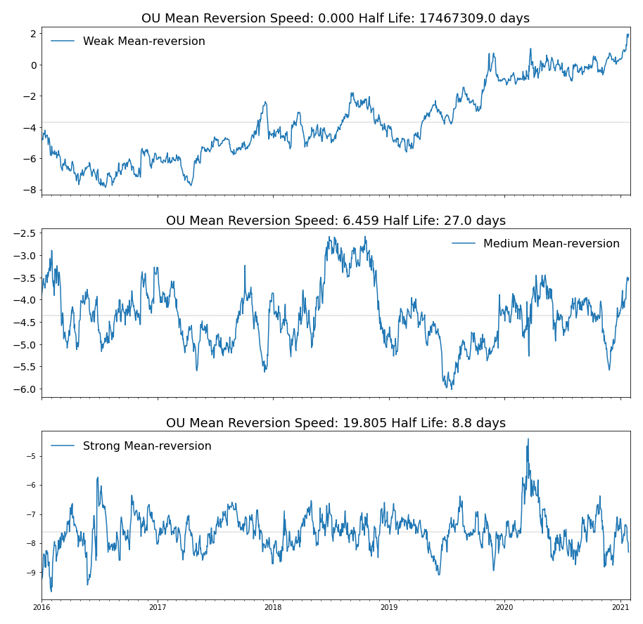
The clustering results have shown that a 15-asset cluster and an 8-asset cluster have been formed with this data set. To demonstrate Box-Tiao canonical decomposition, I have chosen the 8-asset cluster due to its smaller size. Three portfolios have been built according to the Box-Tiao weights as shown in Figure 9 ranging from the least mean-reverting to the most mean-reverting.

Figure 9. Box-Tiao canonical decomposition results.

The results have shown that the least mean-reverting portfolio have shown a persistent upward drift and thus might be suitable for a momentum strategy. This is further corroborated by the fact that the portfolio value process cannot be fit by an OU model according to its abnormally long mean-reversion half-life. The most mean-reverting portfolio, on the other hand, looks noisy; it would take approximately two weeks for the portfolio value to come back half way toward its long-term mean. Depending on the desired trading frequency, a statistical arbitrageur could either choose the most mean-reverting portfolio for more action, or he/she could use a portfolio with moderate predictability for a less noisy portfolio to avoid chopping.

Let’s take a look at the weights for these three portfolios.

Asset
⠀
⠀
ECH
EWP
EWU
EZA
THD
GXG
EWS
EWO

⠀
Least
mean-reverting
-0.300885
-0.263137
-0.006681
-0.027801
0.046753
-0.185164
0.128065
0.886869

Weights
Moderate
mean-reverting
0.070991
-0.441379
0.462643
-0.020616
-0.042529
0.016147
-0.617560
0.449702

⠀
Most
mean-reverting
0.104442
-0.152039
-0.640490
-0.105541
-0.109448
0.259847
0.666222
0.145805

The weights of the least mean-reverting portfolio have shown that it is heavily overweight Austria equities (EWO). The behavior of the portfolio was dominated by this single asset and it is rather unsurprising that the portfolio value has shown non-stationarity, or momentum-like behavior. The most mean-reverting portfolio in this specific example happens to be able to get grouped into four pairs, i.e. Singapore (EWS) – UK (EWU), Austria (EWO) – Spain (EWP), Chile (ECH) – South Africa (EZA), Colombia (GXG) – Thailand (THD). The moderate mean-reverting portfolio, however, has four weights that are considerably smaller than the others; so it can be approximately regarded as a four-asset portfolio that focuses on European equities (EWP, EWU, EWO). The mean-reverting portfolios were constructed based only on price data, but the results made sense financially. For example, the equities from the same region were grouped together as in the moderate mean-reverting portfolio; or the equities from the commodity exporters were paired with each other (Chile is a major copper miner and South Africa is a major platinum and palladium miner) as in the most mean-reverting portfolio. This suggests the sparse estimate of covariance matrix and VAR(1) coefficients can successfully isolate the conditional dependencies between the assets and make use of this information to form mean-reverting portfolios.

A few tips:

Lasso methods are sensitive to the data scales. Therefore, the data have to be standardized before model fitting. This is achieved by setting the option use_standardized=True for the fitting functions.
The sparsity of the covariance matrix is the determining factor of the size of the clusters. It is recommended to set a high regularization parameter for the graphical Lasso model to make sure the graph of the inverse covariance matrix $\Gamma_0^{-1}$ is sufficiently disconnected.
Box-Tiao method is not the only method to use after narrowing down the investing universe. You can still use the greedy algorithm and the convex relaxation approach on the smaller asset clusters.

Greedy Algorithm

The most straightforward approach needs minimal introduction. Let’s directly jump into the codes.

# Calculate least-square VAR(1) estimate and sample covariance
full_var_est = etf_sparse_portf.least_square_VAR_fit(use_standardized=False)
full_cov_est = etf_sparse_portf.autocov(0, use_standardized=False)

# Use greedy algorithm to calculate portfolio weights
greedy_weight = etf_sparse_portf.greedy_search(8, full_var_est, 
                                               full_cov_est, maximize=False)

Three lines of codes are all you need to get a greedy algorithm running using ArbitrageLab. To demonstrate the power of the greedy algorithm, I did not do clustering and took all 45 assets as the investing universe; the covariance estimate and the VAR(1) coefficient matrix estimate were also dense. To make sure we are not comparing apples to oranges, the target cardinality of the portfolio was set to 8.

Let’s take a look at the portfolio formed by this approach.

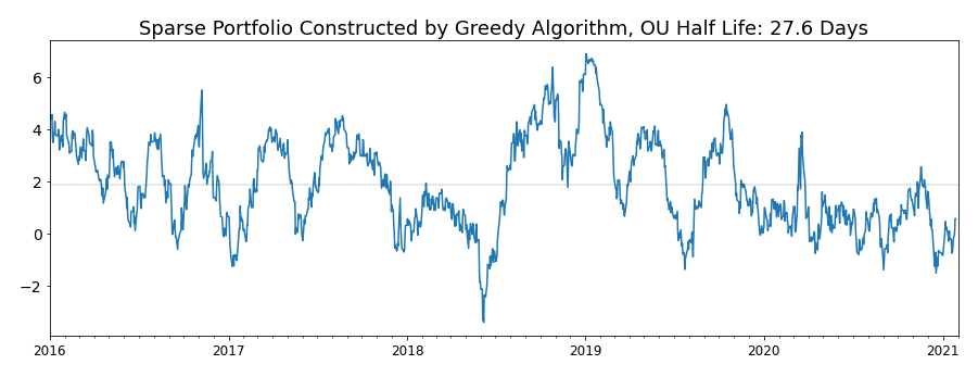
Figure 10. Sparse mean-reverting portfolio built by greedy algorithm.

Asset
EGPT
ARGT
EWZ
EWW
GXG
ECH
EWY
TUR

Weights
-0.035084
-0.332868
0.206248
0.504653
-0.680563
0.315425
-0.026486
-0.165515

The mean-reverting portfolio selected by greedy algorithm looks great for a strategy of lower frequency as the OU half-life of the portfolio is about a month. While the asset clustering method focused on the European region, the greedy algorithm preferred the Latin America region by selecting Argentina (ARGT), Brazil (EWZ), Mexico (EWW), Colombia (GXG), and Chile (ECH) equities in the portfolio. The contribution from Egypt (EGPT), South Korea (EWY), and Turkey (TUR) equities were relatively small. Both the mean-reversion strength and the interpretability of the portfolio built by the greedy algorithm looks promising. Especially, the portfolio did not fall on its face during the market turbulence in early 2020.

Convex Relaxation

Although the convex relaxation looked complicated in theory, in practice it is rather straightforward with the help of ArbitrageLab. Let’s see the code!

Similarly to the setup in the greedy algorithm demonstration, the SDP approach was directly applied to all 45 assets in the investing universe. To set a portfolio variance threshold, a fraction of the median variance of all the asset prices were used, which could be readily calculated with the diagonal of the covariance matrix. Again, the cardinality of the portfolio was set to 8 for a fair comparison.

# Retrieve the median variance of all the asset prices
cov = etf_sparse_portf.autocov(0, use_standardized=False)
var_median = np.median(np.diag(cov))  # Median variance is 16.1

# Use c30% of the median variance as the portfolio variance lower bound, which is 5
sdp_pred_vol_result = etf_sparse_portf.sdp_predictability_vol(rho=0.001, variance=5,
                                                              max_iter=5000,
                                                              use_standardized=False,
                                                              verbose=False)

# Deflate the optimization result into a weight vector
sdp_pred_vol_weights = etf_sparse_portf.sparse_eigen_deflate(sdp_pred_vol_result,
                                                             8, verbose=False)

What did the mean-reverting portfolio look like?

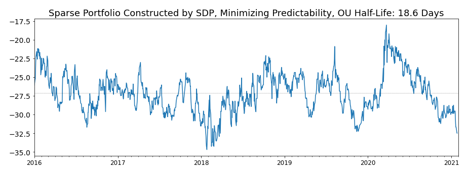
Figure 11. Sparse mean-reverting portfolio built by convex relaxation approach. Predictability is minimized to obtain this portfolio.

Asset
EGPT
ENZL
EZA
GXC
EPU
ARGT
EIS
ECH

Weights
0.114472
-0.171927
-0.754660
-0.089197
0.112914
0.503596
-0.081626
0.326876

Compared to the portfolio constructed by greedy algorithm, this one built by the convex relaxation approach has stronger mean reversion but is slightly noisier. The portfolio focuses on commodity exporters such as New Zealand (ENZL), South Africa (EZA), Peru (EPU), Argentina (ARGT), and Chile (ECH) equities, but its interpretability is worse than the greedy algorithm portfolio as China (GXC), Egypt (EGPT), and Israel equities (EIS) are also included in the portfolio with considerable weights. The volatility of the portfolio is also greater than the greedy algorithm one thanks to the volatility constraint.

Again, a few tips:

Since the SDP result is almost never a rank-one matrix, it is necessary to run sparse_eigen_deflate function to retrieve the leading sparse eigenvector as the portfolio weight.
How do we know if the regularization parameter $\rho$ was set properly? Check the leading sparse eigenvector. Let’s take the portfolio we just obtained as an example. The cardinality of the portfolio was set to 8. If a few weights are orders of magnitude smaller than the others, then a smaller $\rho$ should be used.
You may have noticed that in both greedy algorithm and convex relaxation approach, the data have only been centered to zero mean. Greedy algorithm is more robust and cares less about the scale of the data, but convex relaxation approach may sometimes run into numerical issues, especially for data that are significantly different in the scale. For example, if you would like to build a mean-reverting portfolio out of a group of emerging-market (EM) FX rate against USD, having USDIDR in your portfolio might cause problems (1 USD $\approx$ 14,000 IDR, but 1 USD $\approx$ 7 TRY, for example). In this case, it might be worthwhile to try standardized data by setting use_standardized=True and see if the resulting mean-reverting portfolio is tradable.

Conclusions

This article has covered the sparse mean-reverting portfolio selection problem in depth. Choosing the correct markets to trade are crucial for any trading strategies. Here the focus is to introduce tools for statistical arbitrageurs to build a multi-asset basket from a large number of candidates for mean-reversion trading strategies, but concepts like predictability can be helpful for selecting markets for momentum strategies as well.

Key Takeaways

The mean-reverting portfolios should have as few assets as possible, or sparse in short. Sparse mean-reverting portfolios have better P&L interpretability, use less leverage, and incur fewer transaction costs.
The mean-reversion speed of the Ornstein-Uhlenbeck model directly measures mean-reversion strength but is hard to optimize with respect to portfolio weights. Therefore, mean-reversion proxies like predictability, portmanteau statistic, and crossing statistic are used in the sparse mean-reverting portfolio selection problem.
Stronger mean-reversion is equivalent to less predictability, smaller portmanteau statistic, and higher crossing statistic.
Momentum strategies can be applied to portfolios with high predictability.
Greedy algorithm is a robust method to build sparse mean-reverting portfolios.
Convex relaxation approach offers more control over the sparse mean-reverting portfolio at the cost of model simplicity.
Covariance selection and structured VAR(1) estimate with Lasso models can help find smaller asset clusters. This can be regarded as a preprocessing step, for Box-Tiao canonical decomposition, greedy algorithm, and convex relaxation approach can all be used on the these clusters to construct a sparse mean-reverting portfolio.

References

Footnotes

The data used are daily data of 45 international equity ETFs starting from Jan 1st, 2016 to Jan 27th, 2021. The details of these ETFs can be downloaded here as an Excel spreadsheet.
$\binom{505}{5} = 268,318,178,226$ just in case you are wondering.

References

- Box, G.E. and Tiao, G.C., 1977. A canonical analysis of multiple time series. Biometrika, 64(2), pp.355-365.
- d’Aspremont, A., 2011. Identifying small mean-reverting portfolios. Quantitative Finance, 11(3), pp.351-364.
- Fogarasi, N. and Levendovszky, J., 2012. Improved parameter estimation and simple trading algorithm for sparse, mean-reverting portfolios. In Annales Univ. Sci. Budapest., Sect. Comp, 37, pp. 121-144.
- Ghojogh, B., Karray, F. and Crowley, M., 2019. Eigenvalue and generalized eigenvalue problems: Tutorial. arXiv preprint arXiv:1903.11240.
- Gilbert, J.R., 1994. Predicting structure in sparse matrix computations. SIAM Journal on Matrix Analysis and Applications, 15(1), pp.62-79.
- Kedem, B. and Yakowitz, S., 1994. Time series analysis by higher order crossings (pp. 115-143). New York: IEEE press.
- Ljung, G.M. and Box, G.E., 1978. On a measure of lack of fit in time series models. Biometrika, 65(2), pp.297-303.
- Natarajan, B.K., 1995. Sparse approximate solutions to linear systems. SIAM journal on computing, 24(2), pp.227-234.
- Yuan, X.T. and Zhang, T., 2013. Truncated Power Method for Sparse Eigenvalue Problems. Journal of Machine Learning Research, 14(4).